In this blog, we'll cover:

• An introduction to LangChain and show why it’s awesome.

• An explanation of how Ray complements LangChain by: 

  • Showing how with a few minor changes, we can speed parts of the process up by a factor of 4x or more

  • Making LangChain’s capabilities available in the cloud using Ray Serve

  • Using self-hosted models by running Ray Serve, LangChain and the model all in the same Ray cluster without having to worry about maintaining individual machines.

LinkIntroduction

Ray is a very powerful framework for ML orchestration, but with great power comes voluminous documentation. 120 megabytes in fact. How can we make that documentation more accessible?

Answer: make it searchable! It used to be that creating your own high quality search results was hard. But by using LangChain, we can build it in about 100 lines of code. 

This is where LangChain comes in. LangChain provides an amazing suite of tools for everything around LLMs. It’s kind of like HuggingFace but specialized for LLMs. There are tools (chains) for prompting, indexing, generating and summarizing text. While an amazing tool, using Ray with it can make LangChain even more powerful. In particular, it can: 

• Simply and quickly help you deploy a LangChain service. 

• Rather than relying on remote API calls, allow Chains to run co-located and auto-scalable with the LLMs itself. This brings all the advantages we discussed in a previous blog post: lower cost, lower latency, and control over your data.

LinkBuilding the LangChain index

Build a document index easily with Ray and Langchain

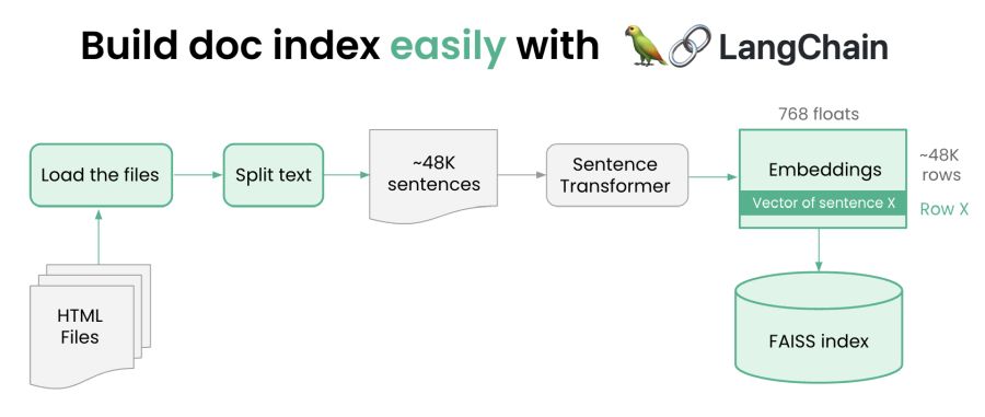
First we will build the index via the following steps. 

1. Download the content we want to index locally. 

2. Read the content and cut it into tiny little pieces (about a sentence each). This is because it is easier to match queries against pieces of a page rather than the whole page.

3. Use the Sentence Transformers library from HuggingFace to generate a vector representation of each sentence. 

4. Embed those vectors in a Vector database (we use FAISS, but you could use whatever you like). 

The amazing thing about this code is how simple it is - See Here. As you will see, thanks to LangChain, all the heavy lifting is done for us. Let’s pick a few excerpts. 

Assuming we’ve downloaded the Ray docs, this is all we have to do to read all the docs in:

1loader = ReadTheDocsLoader("docs.ray.io/en/master/")
2docs = loader.load() 

The next step is to break each document into little chunks. LangChain uses splitters to do this. So all we have to do is this:

1chunks = text_splitter.create_documents(
2    [doc.page_content for doc in docs], 
3    metadatas=[doc.metadata for doc in docs])

We want to preserve the metadata of what the original URL was, so we make sure to retain the metadata along with these documents. 

Now we have the chunks we can embed them as vectors. LLM providers do offer APIs for doing this remotely (and this is how most people use LangChain). But, with just a little bit of glue we can download Sentence Transformers from HuggingFace and run them locally (inspired by LangChain’s support for llama.cpp). Here’s the glue code. 

By doing so, we reduce latency, stay on open source technologies, and don’t need a HuggingFace key or to pay for API usage. 

Finally, we have the embeddings, now we can use a vector database – in this case FAISS – to store the embeddings. Vector databases are optimized for doing quick searches in high dimensional spaces. Again, LangChain makes this effortless.

1from langchain.vectorstores import FAISS
2
3db = FAISS.from_documents(chunks, embeddings)
4db.save_local(FAISS_INDEX_PATH)

And that’s it. The code for this is here. Now we can build the store.

1% python build_vector_store.py

This takes about 8 minutes to execute. Most of that time is spent doing the embeddings. Of course, it’s not a big deal in this case, but imagine if you were indexing hundreds of gigabytes instead of hundreds of megabytes.

LinkAccelerating indexing using Ray

[Note: This is a slightly more advanced topic and can be skipped on first reading. It just shows how we can do it more quickly – 4x to 8x times more quickly]

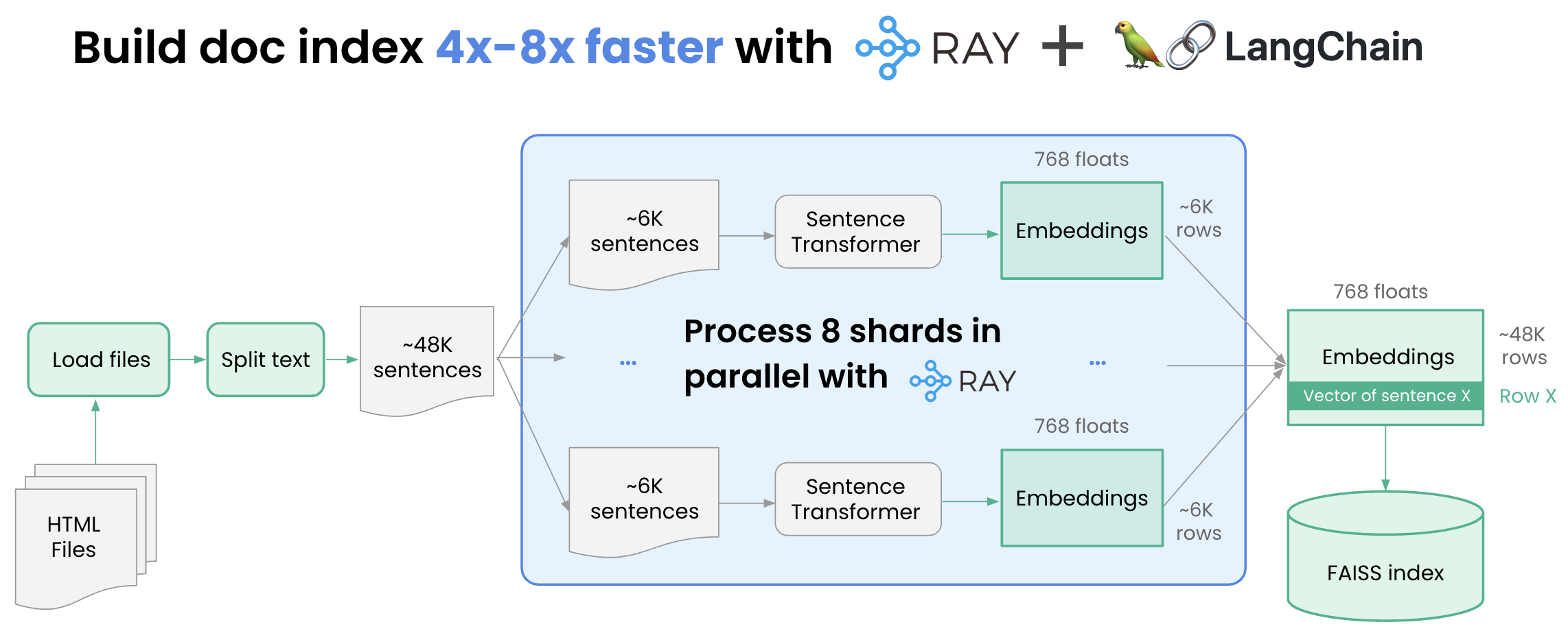
How can we speed up indexing? The great thing is that embedding is easy to parallelize. What if we: 

1. Sliced the list of chunks into 8 shards. 

2. Embedded each of the 8 shards separately.

3. Merge the shards. 

Build a document index 4-8x faster with Ray

One key thing to realize is that embedding is GPU accelerated, so if we want to do this, we need 8 GPUs. Thanks to Ray, those 8 GPUS don’t have to be on the same machine. But even on a single machine, there are significant advantages to using Ray. And one does not have to go to the complexity of setting up a Ray cluster, all you need to do is pip install ray[default] and then import ray. 

This requires some minor surgery to the code. Here’s what we have to do.

First, create a task that creates the embedding and then uses it to index a shard. Note the Ray annotation and us telling us each task will need a whole GPU.

1@ray.remote(num_gpus=1)
2def process_shard(shard): 
3    embeddings = LocalHuggingFaceEmbeddings('multi-qa-mpnet-base-dot-v1')
4    result = FAISS.from_documents(shard, embeddings)
5    return result
6

Next, split the workload in the shards. NumPy to the rescue! This is a single line: 

1shards = np.array_split(chunks, db_shards)

Then, create one task for each shard and wait for the results.

1futures = [process_shard.remote(shards[i]) for i in range(db_shards)]
2results = ray.get(futures)

Finally, let’s merge the shards together. We do this using simple linear merging. 

1db = results[0]
2for i in range(1,db_shards):
3    db.merge_from(results[i])

Here’s what the sped up code looks like.

You might be wondering, does this actually work? We ran some tests on a g4dn.metal instance with 8 GPUs. The original code took 313 seconds to create the embeddings, the new code took 70 seconds, that’s about a 4.5x improvement. There’s still some one-time overheads to creating tasks, setting up the GPUs etc. This reduces as the data increases. For example, we did a simple test with 4 times the data, and it was around 80% of the theoretical maximum performance (ie. 6.5x faster vs theoretical maximum of 8x faster from the 8 GPUs). 

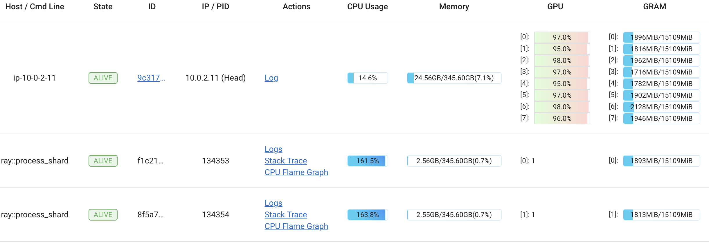
We can use the Ray Dashboard to see how hard those GPUs are working. Sure enough they’re all close to 100% running the process_shard method we just wrote.

Dashboard shows that GPU utilization is maxed out across all instances

It turns out merging vector databases  is pretty fast, taking only 0.3 seconds for all 8 shards to be merged. 

LinkServing

Serve search queries with Ray and Langchain

Serving is another area where the combination of LangChain and Ray Serve shows its power. This is just scratching the surface: we’ll explore amazing capabilities like independent auto scaling and request batching in our next blog post in the series.

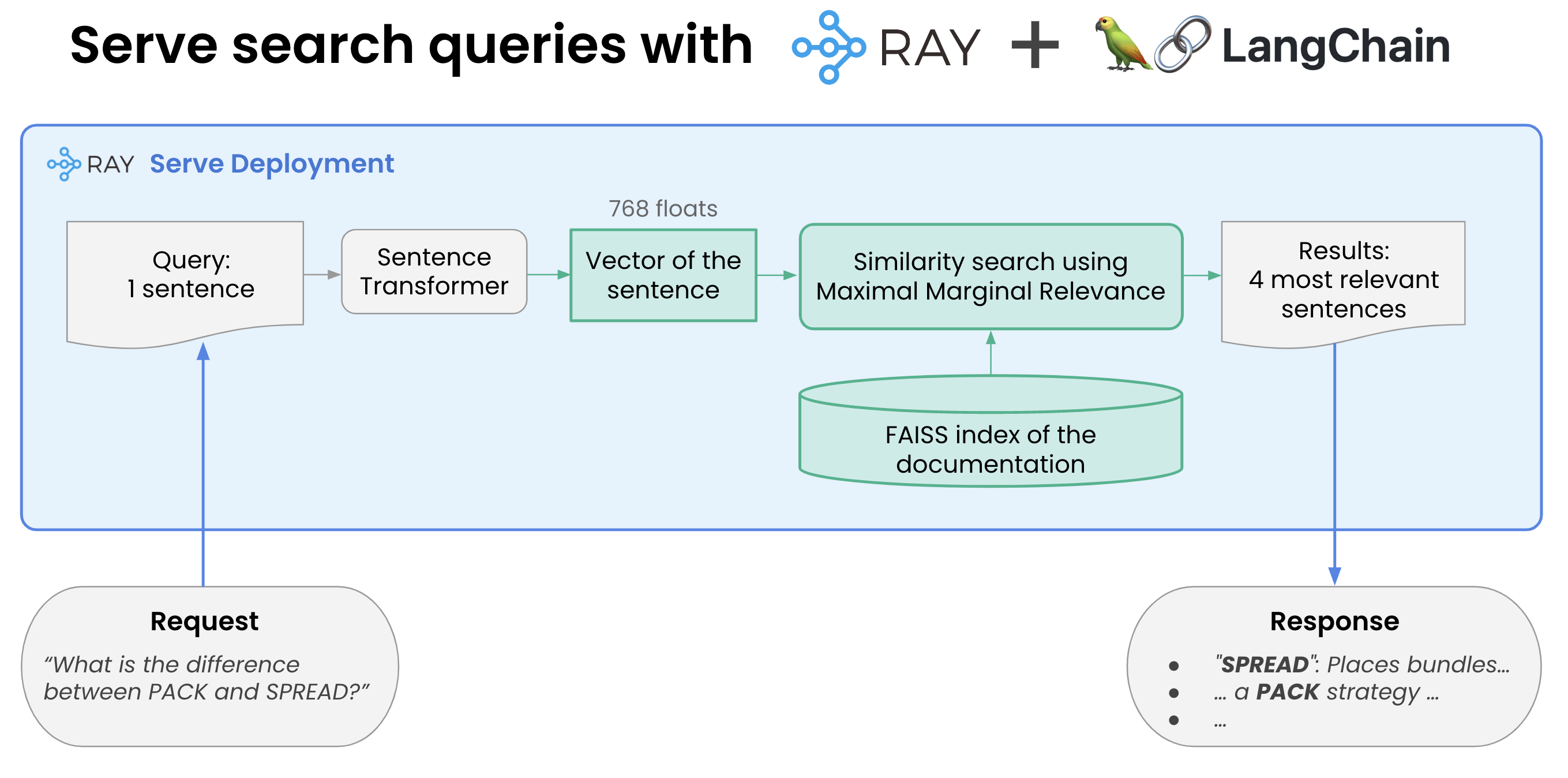
The steps required to do this are:

1. Load the FAISS database we created and the instantiate the embedding

2. Start using FAISS to do similarity searches.

Ray Serve makes this magically easy. Ray uses a “deployment” to wrap a simple python class. The __init__ method does the loading and then __call__ is what actually does the work. Ray takes care of connecting it to the internet, bringing up a service, http and so on.

Here’s a simplified version of the code:

1@serve.deployment
2class VectorSearchDeployment:
3    def __init__(self):
4        self.embeddings = … 
5        self.db = FAISS.load_local(FAISS_INDEX_PATH, self.embeddings)
6
7    def search(self,query): 
8        results = self.db.max_marginal_relevance_search(query)
9        retval = <some string processing of the results>
10        return retval
11
12    async def __call__(self, request: Request) -> List[str]:
13        return self.search(request.query_params["query"])
14
15deployment = VectorSearchDeployment.bind()

That’s it!

Let’s now start this service with the command line (of course Serve has more deployment options than this, but this is an easy way):

1% serve run serve_vector_store:deployment

Now we can write a simple python script to query the service to get relevant vectors(it’s just a web server running on port 8000).

1import requests
2import sys
3query = sys.argv[1]
4response = requests.post(f'http://localhost:8000/?query={query}')
5print(response.content.decode())

And now let’s try it out:

1$ python query.py 'Does Ray Serve support batching?'
2From http://docs.ray.io/en/master/serve/performance.html
3
4You can check out our microbenchmark instructions
5to benchmark Ray Serve on your hardware.
6Request Batching#
7====
8
9From http://docs.ray.io/en/master/serve/performance.html
10
11You can enable batching by using the ray.serve.batch decorator. Let’s take a look at a simple example by modifying the MyModel class to accept a batch.
12from ray import serve
13import ray
14@serve.deployment
15class Model:
16    def __call__(self, single_sample: int) -> int:
17        return single_sample * 2
18====
19
20From http://docs.ray.io/en/master/ray-air/api/doc/ray.train.lightgbm.LightGBMPredictor.preferred_batch_format.html
21
22native batch format.
23DeveloperAPI: This API may change across minor Ray releases.
24====
25
26From http://docs.ray.io/en/master/serve/performance.html
27
28Machine Learning (ML) frameworks such as Tensorflow, PyTorch, and Scikit-Learn support evaluating multiple samples at the same time.
29Ray Serve allows you to take advantage of this feature via dynamic request batching.
30====

LinkConclusion

We showed in the above code just how easy it is to build key components of an LLM-based search engine and serve its responses to the entire world by combining the power of LangChain and Ray Serve. And we didn’t have to deal with a single pesky API key! 

Tune in for Part 2, where we will show how to turn this into a chatgpt-like answering system. We’ll use open source LLMs like Dolly 2.0 to do that. 

And finally we’ll share Part 3 where we’ll talk about scalability and cost. The above is fine for a few hundred queries per second, but what if you need to scale to a lot more? And are the claims about latency correct?

LinkNext Steps

See part 2 here.

Review the code and data used in this blog in the following Github repo.

See our earlier blog series on solving Generative AI infrastructure with Ray.

If you are interested in learning more about Ray, see Ray.io and Docs.Ray.io.

To connect with the Ray community join #LLM on the Ray Slack or our Discuss forum.

If you are interested in our Ray hosted service for ML Training and Serving, see Anyscale.com/Platform and click the 'Try it now' button

Ray Summit 2023: If you are interested to learn much more about how Ray can be used to build performant and scalable LLM applications and fine-tune/train/serve LLMs on Ray, join Ray Summit on September 18-20th! We have a set of great keynote speakers including John Schulman from OpenAI and Aidan Gomez from Cohere, community and tech talks about Ray as well as practical training focused on LLMs.