Gradient boosting algorithms are widely used in supervised learning. While they are powerful, they can take a long time to train. Extreme gradient boosting, or XGBoost, is an open-source implementation of gradient boosting designed for speed and performance. However, even XGBoost training can sometimes be slow. 

There are quite a few approaches to accelerating this process like: 

• Changing tree construction method

• Leveraging cloud computing

• Distributed XGBoost on Ray

This article will review the advantages and disadvantages of each approach as well as go over how to get started.

LinkChanging your tree construction algorithm

XGBoost’s tree_method parameter allows you to specify which tree construction algorithm you want to use. Choosing an appropriate tree construction algorithm (exact, approx, hist, gpu_hist, auto) for your problem can help you produce an optimal model faster. Let’s now review the algorithms.

exact

It is an accurate algorithm, but it is not very scalable as during each split find procedure it iterates over all entries of input data. In practice, this means long training times. It also doesn’t support distributed training. You can learn more about this algorithm in the original XGBoost paper. 

approx

While the exact algorithm is accurate, it is inefficient when the data does not completely fit into memory. The approximate tree method from the original XGBoost paper uses quantile sketch and gradient histograms.

hist

An approximation tree method used in LightGBM with slight differences in implementation (uses some performance improvements such as bins caching) from approx. This is typically faster than approx. 

gpu_hist

As GPUs are critical for many machine learning applications, XGBoost has a GPU implementation of the hist algorithm gpu_hist) that has support for external memory. It is much faster and uses considerably less memory than hist. Note that XGBoost doesn’t have native support for GPUs on some operating systems.

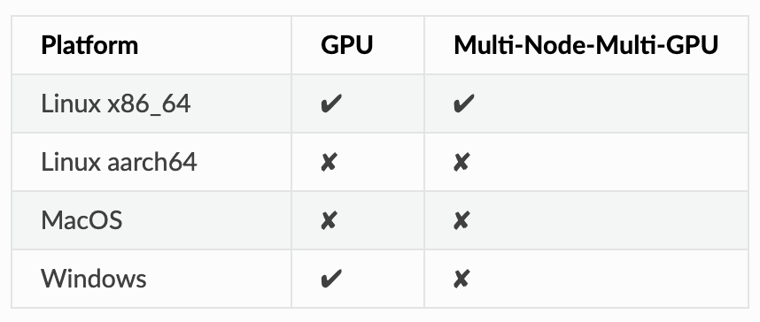XGBoost documentation

auto

This is the default value for the parameter. Based on the dataset size, XGBoost will choose the “fastest method”. For small datasets, exact will be used. For larger datasets, approx will be used. Note that hist and gpu_hist aren’t considered in this heuristic based approach even though they are often faster. 

If you run this code, you will see how running models using gpu_hist can save a lot of time. On a relatively small dataset (100,000 rows, 1000 features) on my computer, changing from hist to gpu_hist decreased training time by about a factor of 2.

LinkLeveraging cloud computing

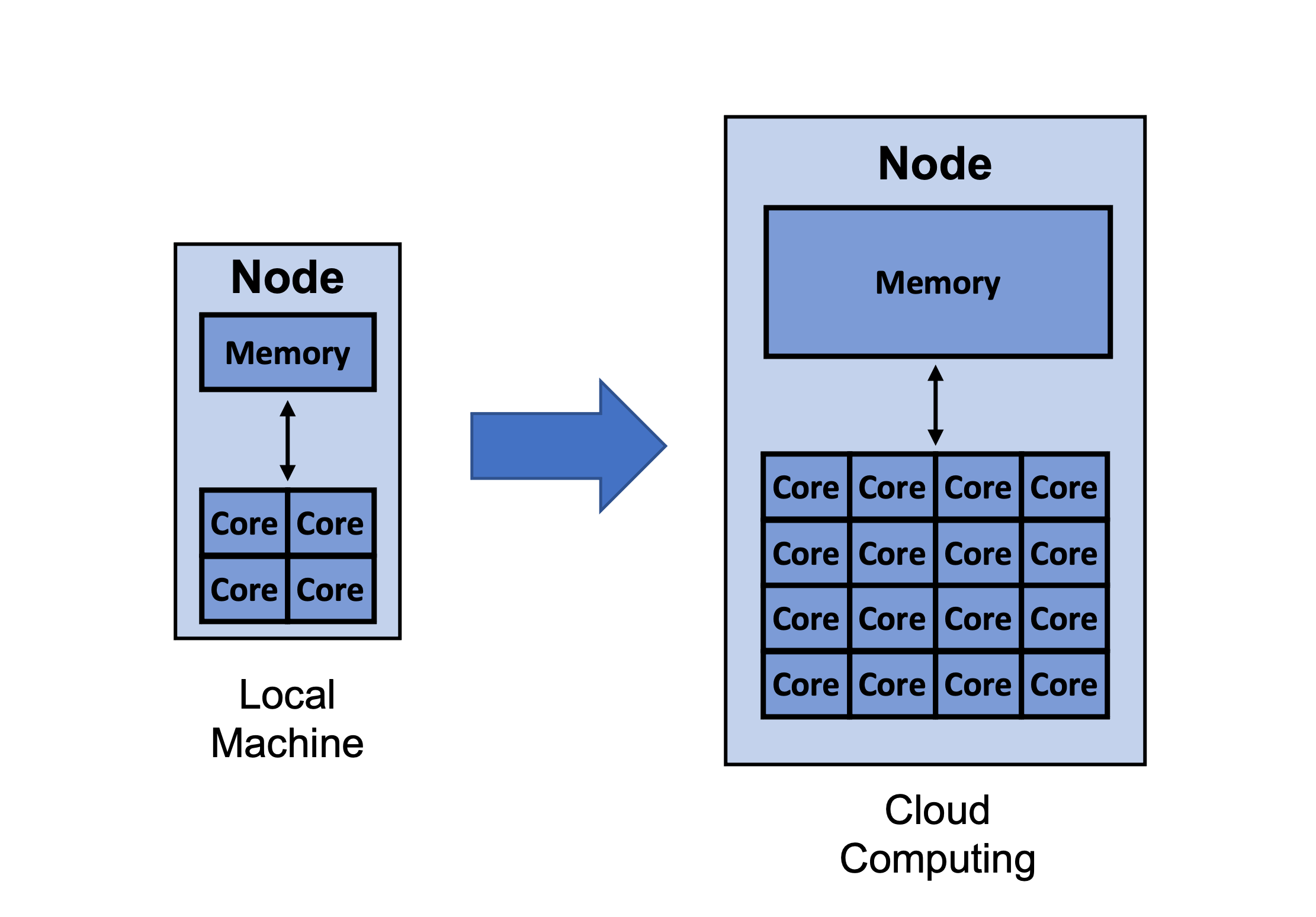Cloud computing allows you to not only utilize more cores and memory than your local machine, but can also give you access to specialized resources like GPUs.

The last section was mostly about choosing more efficient algorithms in order to better use of available computational resources. However, sometimes available computational resources are not enough and you simply need more. For example, the MacBook shown in the image below only has 4 cores and 16GB memory. Furthermore, it runs on MacOS which at the time of this writing, XGBoost doesn’t have GPU support for.

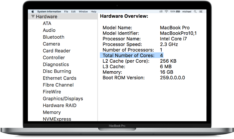For the purpose of this post, you can think of the MacBook above as a single node with 4 cores.

A way around this problem is to utilize more resources on the cloud. Utilizing cloud providers aren’t free, but they often allow you to utilize more cores and memory than your local machine. Additionally, if XGBoost doesn’t have support for your local machine, it is easy to choose an instance type that XGBoost has GPU support for. 

If you would like to try speeding up your training on the cloud, below is an overview of the steps from Jason Brownlee’s article on how to train an XGBoost model on an AWS EC2 instance:

1. Setup an AWS account (if needed)

2. Launch an AWS Instance

3. Login and run the code

4. Train an XGBoost model

5. Close the AWS Instance (only pay for the instance when you are using it)

If you select a more powerful instance than what you have locally, you’ll likely see that training on the cloud is faster. Note that multi-GPU training with XGBoost actually requires distributed training which means you need more than a single node/instance to accomplish this. 

LinkDistributed XGBoost Training with Ray

So far, this tutorial has covered speeding up training by changing the tree construction algorithm and by increasing computing resources through cloud computing. Another solution is to distribute XGBoost model training with XGBoost-Ray which leverages Ray.

LinkWhat is Ray?

Ray is a fast, simple distributed execution framework that makes it easy to scale your applications and to leverage state of the art machine learning libraries. Using Ray, you can take Python code that runs sequentially and with minimal code changes transform it into a distributed application. If you would like to learn about Ray and the actor model, you can learn about it here. 

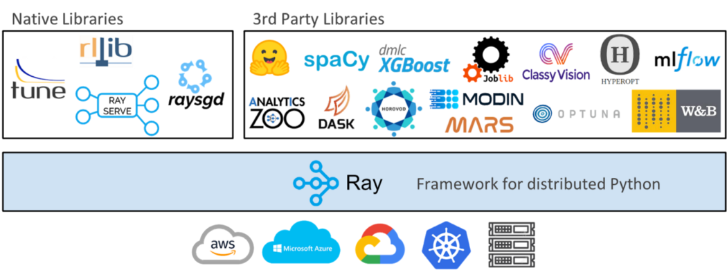While this tutorial explores how Ray makes it easy to parallelize and distribute XGBoost code, it is important to note that Ray and its ecosystem also make it easy to distribute plain Python code as well as existing libraries like scikit-learn, LightGBM, PyTorch, and much more.

LinkHow to get started with XGBoost-Ray

To get started with XGBoost-Ray, you first need to install it.

pip install "xgboost_ray"

Since it is fully compatible with the core XGBoost API, all you need is a few code changes to scale XGBoost training from a single machine to a cluster with hundreds of nodes.

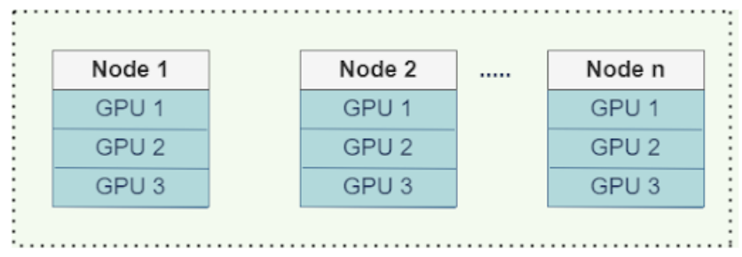XGBoost-Ray supports multi-node/multi-GPU training. On a machine, GPUs communicate gradients via NCCL2. Between nodes, they use Rabit instead ​​(learn more).

As you can see in the code below, the API is very similar to XGBoost. The highlighted portions are where the code is different than the normal XGBoost API.

1from xgboost_ray import RayXGBClassifier, RayParams
2from sklearn.datasets import load_breast_cancer
3from sklearn.model_selection import train_test_split
4
5seed = 42
6
7X, y = load_breast_cancer(return_X_y=True)
8X_train, X_test, y_train, y_test = train_test_split(
9    X, y, train_size=0.25, random_state=42
10)
11
12clf = RayXGBClassifier(
13    n_jobs=4,  # In XGBoost-Ray, n_jobs sets the number of actors
14    random_state=seed)
15
16# scikit-learn API will automatically convert the data
17# to RayDMatrix format as needed.
18# You can also pass X as a RayDMatrix, in which case
19# y will be ignored.
20
21clf.fit(X_train, y_train)
22
23pred_ray = clf.predict(X_test)
24print(pred_ray)
25
26pred_proba_ray = clf.predict_proba(X_test)
27print(pred_proba_ray)

The code above shows how little you need to change your code to use XGBoost-Ray. While you don’t need XGboost-Ray to train the breast cancer dataset, a previous post ran benchmarks on several dataset sizes (~1.5M to ~12M rows) across different amounts of workers (1 to 8) to show how it performs on bigger datasets on a single node.

Training times for single node benchmarks (lower is better). XGBoost-Ray and XGBoost-Dask achieve similar performance on a single AWS m5.4xlarge instance with 16 cores and 64 GB memory.

XGBoost-Ray is also performant in multi-node (distributed) settings as the image below shows.

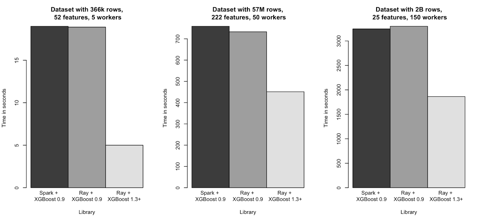Multi-node training times on several synthetic dataset sizes ranging from ~400k to ~2B rows (where lower is better). XGBoost-Ray and XGBoost-Spark achieve similar performance.

If you would like to learn more about XGBoost Ray, check out this post on XGBoost-Ray. 

LinkConclusion

This post went over a couple approaches you can use to speed up XGBoost model training like changing tree construction methods, leveraging cloud computing, and distributed XGBoost on Ray. If you have any questions or thoughts about XGBoost on Ray, please feel free to join our community through Discourse or Slack. If you would like to keep up to date with all things Ray, consider following @raydistributed on twitter and sign up for the Ray newsletter.