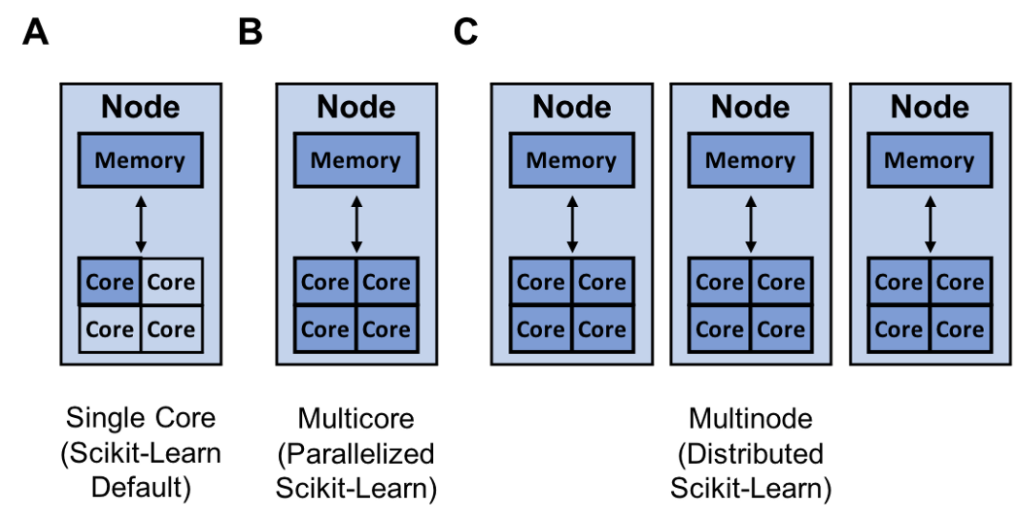Resources (dark blue) that scikit-learn can utilize for single core (A), multicore (B), and multinode training (C)

Scikit-Learn is an easy to use Python library for machine learning. However, sometimes scikit-learn models can take a long time to train. The question becomes, how do you create the best scikit-learn model in the least amount of time? There are quite a few approaches to solving this problem like:

• Changing your optimization function (solver)

• Using different hyperparameter optimization techniques (grid search, random search, early stopping)

• Parallelize or distribute your training with joblib and Ray

This post gives an overview of each approach, discusses some limitations, and offers resources to speed up your machine learning workflow!

LinkChanging your optimization algorithm (solver)

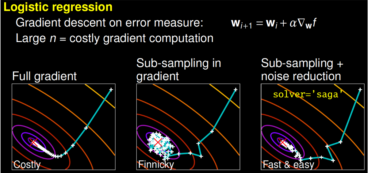Some solvers can take longer to converge. Image from Gaël Varoquaux's talk

Better algorithms allow you to make better use of the same hardware. With a more efficient algorithm, you can produce an optimal model faster. One way to do this is to change your optimization algorithm (solver). For example, scikit-learn’s logistic regression, allows you to choose between solvers like ‘newton-cg’, ‘lbfgs’, ‘liblinear’, ‘sag’, and ‘saga’.

To understand how different solvers work, I encourage you to watch a talk by scikit-learn core contributor Gaël Varoquaux. To paraphrase part of his talk, a full gradient algorithm (liblinear) converges rapidly, but each iteration (shown as a white +) can be prohibitively costly because it requires you to use all of the data. In a sub-sampled approach, each iteration is cheap to compute, but it can converge much more slowly. Some algorithms like ‘saga’ achieve the best of both worlds. Each iteration is cheap to compute, and the algorithm converges rapidly because of a variance reduction technique. It is important to note that quick convergence doesn’t always matter in practice and different solvers suit different problems.

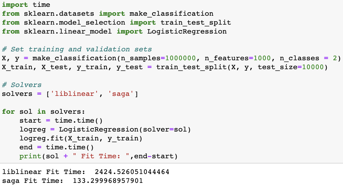
To determine which solver is right for your problem, you can check out the documentation to learn more!

LinkDifferent hyperparameter optimization techniques (grid search, random search, early stopping)

To achieve high performance for most scikit-learn algorithms, you need to tune a model’s hyperparameters. Hyperparameters are the parameters of a model which are not updated during training. They can be used to configure the model or training function. Scikit-Learn natively contains a couple techniques for hyperparameter tuning like grid search (GridSearchCV) which exhaustively considers all parameter combinations and randomized search (RandomizedSearchCV) which samples a given number of candidates from a parameter space with a specified distribution. Recently, scikit-learn added the experimental hyperparameter search estimators halving grid search (HalvingGridSearchCV) and halving random search (HalvingRandomSearch).

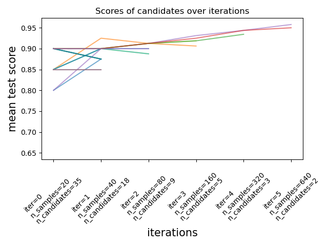Successive halving is an experimental new feature in scikit-learn version 0.24.1 (January 2021). Image from documentation.

These techniques can be used to search the parameter space using successive halving. The image above shows that all hyperparameter candidates are evaluated with a small number of resources at the first iteration and the more promising candidates are selected and given more resources during each successive iteration.

While these new techniques are exciting, there is a library called Tune-sklearn that provides cutting edge hyperparameter tuning techniques (bayesian optimization, early stopping, and distributed execution) that can provide significant speedups over grid search and random search.

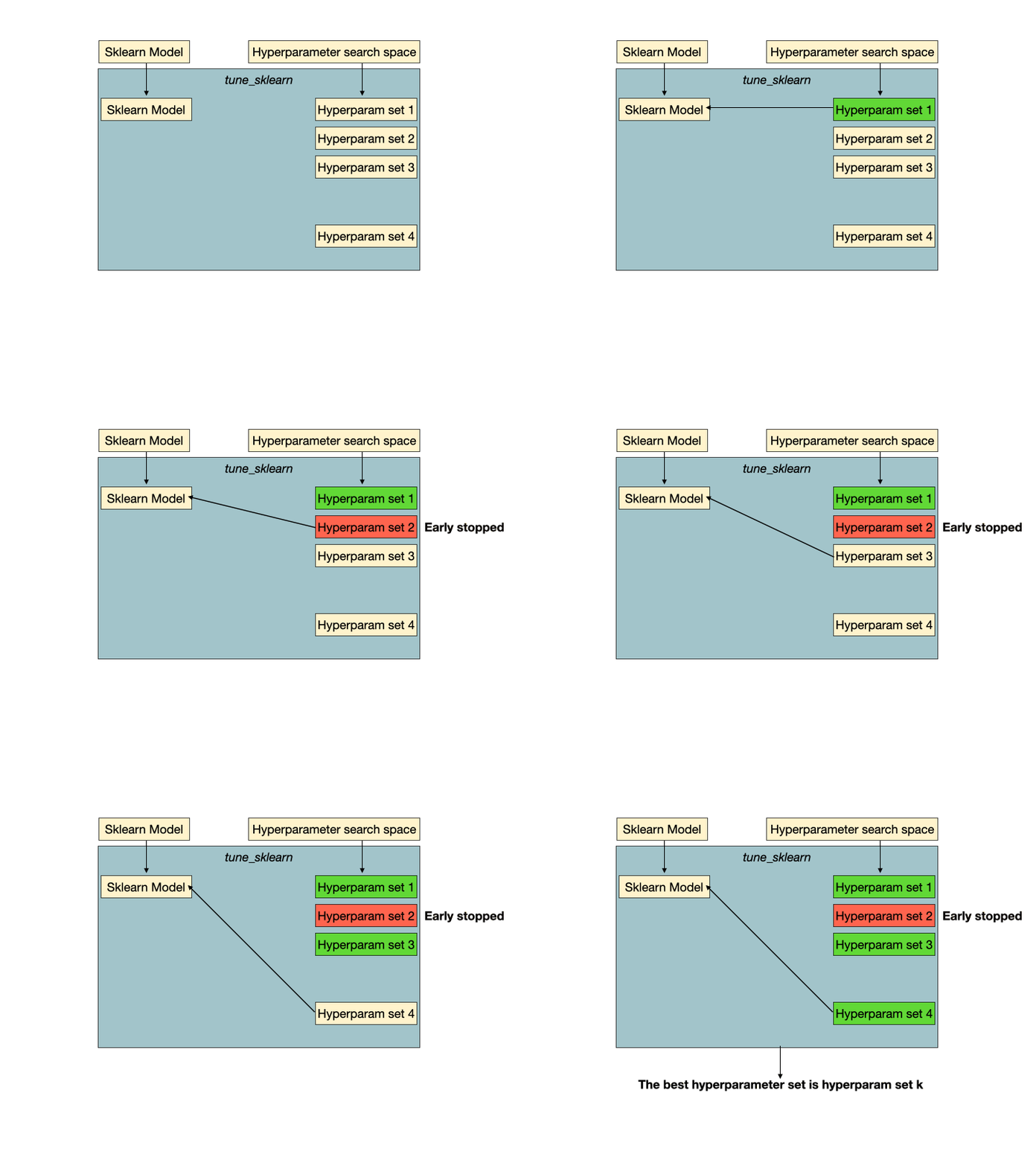Early stopping in action. Hyperparameter set 2 is a set of unpromising hyperparameters that would be detected by Tune-sklearn's early stopping mechanisms, and stopped early to avoid wasting time and resources. Image from GridSearchCV 2.0.

Features of Tune-sklearn include:

• Consistency with the scikit-learn API: You usually only need to change a couple lines of code to use Tune-sklearn (example).

• Accessibility to modern hyperparameter tuning techniques: It is easy to change your code to utilize techniques like bayesian optimization, early stopping, and distributed execution

• Framework support: There is not only support for scikit-learn models, but other scikit-learn wrappers such as Skorch (PyTorch), KerasClassifiers (Keras), and XGBoostClassifiers (XGBoost)

• Scalability: The library leverages Ray Tune, a library for distributed hyperparameter tuning, to efficiently and transparently parallelize cross validation on multiple cores and even multiple machines.

Perhaps most importantly, tune-sklearn is fast as you can see in the image below.

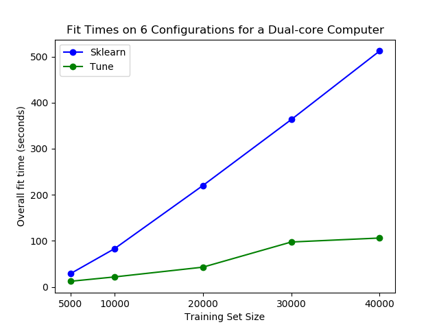You can see significant performance differences on an average laptop using tune-sklearn. Image from GridSearchCV 2.0.

If you would like to learn more about tune-sklearn, you should check out this blog post.

For more on hyperparameters and various tuning approaches, read our three-part blog series on hyperparameter tuning.

LinkParallelize or distribute your training with joblib and Ray

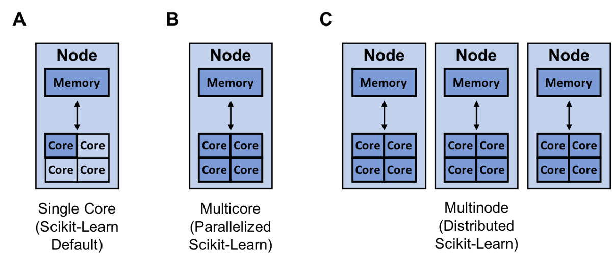Resources (dark blue) that scikit-learn can utilize for single core (A), multicore (B), and multinode training (C)

Another way to increase your model building speed is to parallelize or distribute your training with joblib and Ray. By default, scikit-learn trains a model using a single core. It is important to note that virtually all computers today have multiple cores.

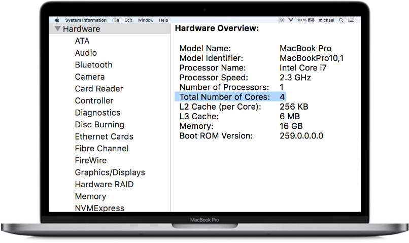For the purpose of this blog, you can think of the MacBook above as a single node with 4 cores.

Consequently, there is a lot of opportunity to speed up the training of your model by utilizing all the cores on your computer. This is especially true if your model has a high degree of high degree of parallelism like a random forest®.

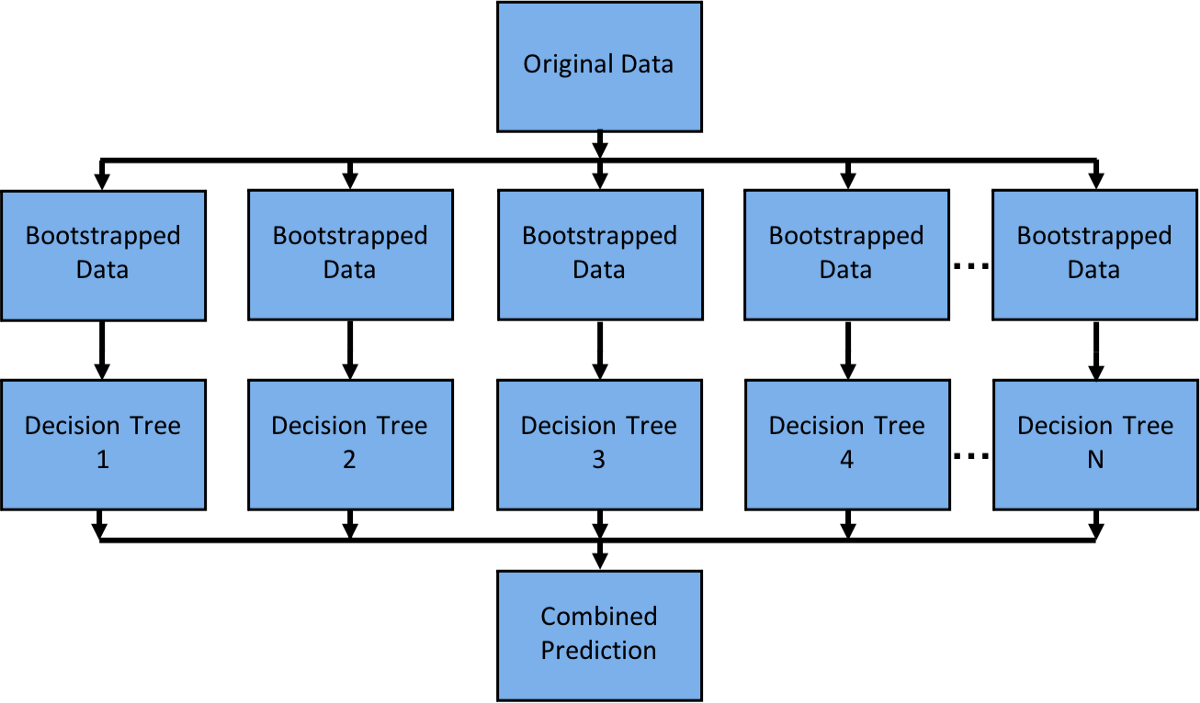A random forest® is an easy model to parallelize as each decision tree is independent of the others.

Scikit-Learn can parallelize training on a single node with joblib which by default uses the ‘loky’ backend. Joblib allows you to choose between backends like ‘loky’, ‘multiprocessing’, ‘dask’, and ‘ray’. This is a great feature as the ‘loky’ backend is optimized for a single node and not for running distributed (multinode) applications. Running distributed applications can introduce a host of complexities like:

• Scheduling tasks across multiple machines

• Transferring data efficiently

• Recovering from machine failures

Fortunately, the ‘ray’ backend can handle these details for you, keep things simple, and give you better performance. The image below shows the normalized speedup in terms of execution time of Ray, Multiprocessing, and Dask relative to the default ‘loky’ backend.

The performance was measured on one, five, and ten m5.8xlarge nodes with 32 cores each. The performance of Loky and Multiprocessing does not depend on the number of machines because they run on a single machine. Image source.

If you would like to learn about how to quickly parallelize or distribute your scikit-learn training, you can check out this blog post

LinkConclusion

This post went over a couple ways you can build the best scikit-learn model possible in the least amount of time. There are some ways that are native to scikit-learn like changing your optimization function (solver) or by utilizing experimental hyperparameter optimization techniques like HalvingGridSearchCV or HalvingRandomSearch. There are also libraries that you can use as plugins like Tune-sklearn and Ray to further speed up your model building. If you have any questions or thoughts about Tune-sklearn and Ray, please feel free to join our community through Discourse or Slack.