In 1949 a British newspaper, The Star, confidently complained in a news article about the EDSAC computer: “The ‘brain’ [computer] may one day come down to our level [of the common people] and help with our income-tax and book-keeping calculations. But this is speculation, and there is no sign of it so far.”

Income-tax and book-keeping aside—computers perhaps were expected to help with demands of heavy calculations back then—today’s top-of-the-line laptops or personal computers, armed with multiple cores and hardware accelerators and retina displays, can carry the burden of astronomical calculations at lightning speed. Not a hyperbole or speculation. But a fact.

In part 1 of this blog series, we shared five considerations for deploying machine learning models in production. This post will elaborate on two concerns: 1) Developing with Ease and 2) Tuning and Training at Scale and Tracking Model Experiments.

LinkDeveloping with ease

For machine learning (ML) workloads, Python has become the de-facto programming language of choice, partly because of its flourishing PyData ecosystem and partly because it is easy to learn. 

Python developers prefer to customize and isolate their developer environments to match their staging or production environment with library dependencies using conda or Python virtual environments. Ideally, as best practice holds, if the same code developed on your laptop can run with minimal changes on a staging or production environment on a cluster, it can immensely improve end-to-end developer productivity. 

Consider developing two machine learning models using two different frameworks: scikit-learn and PyTorch. Both may have Python module dependencies the other may not need, and for development, you may wish not to conflate their environments. You may want to keep the settings distinct for model building, testing, debugging, and validating with small datasets. You may want to move or work in either or both environments concurrently seamlessly. 

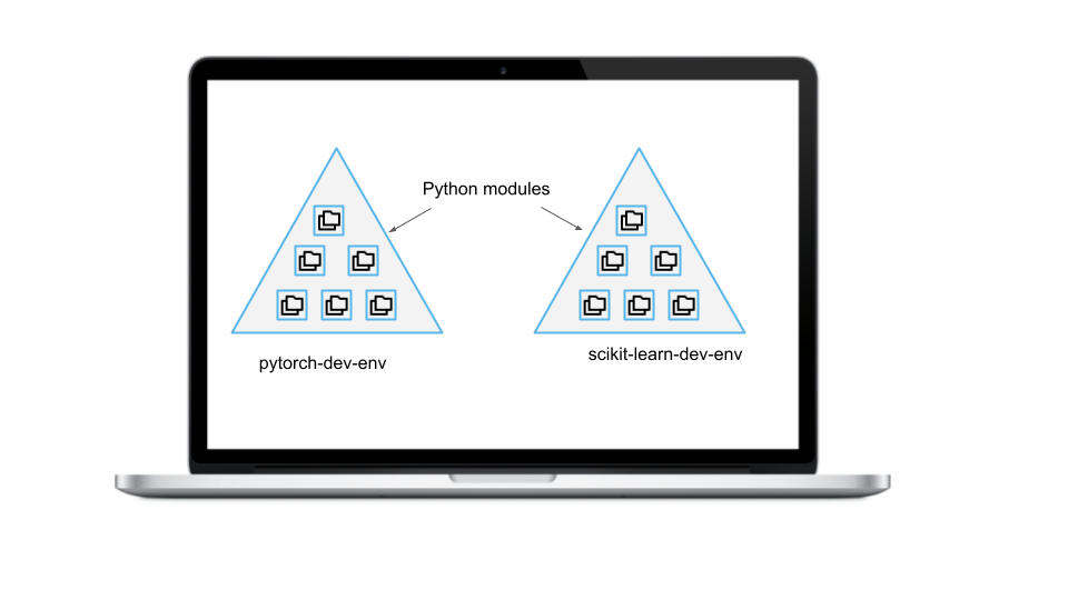Figure 1. Laptop with Python Modules and Conda Development Environments

To achieve this setup, use conda or Python environments. We will use conda here for familiarity:

1. Create two distinct environments_<conda_name>.yml files

2. Create two distinct conda environments and install the required dependencies.

   a. conda create -f environment_pytorch-dev-env.yml

   b. conda create -f environments_scikit-learn-dev-env.yml

3. Activate either of the conda environments

   a. conda activate pytorch-dev-env

4. Use your IDE or Jupyter notebook to develop your models.

An example of one of your conda-specific files, environment_pytorch-dev-env.yml, may look as follows:

1name: pytorch-dev-env
2channels:
3  - conda-forge
4dependencies:
5  - python >= 3.8
6  - pip
7  - numpy >= 1.18.5
8  - pandas
9  - torch
10  - torchvision
11  - tensorboard
12  - mlflow
13- pip:
14    - ray[default, tune]
15    - tensorboard >= 2.3
16    - tensorflow >= 2.3
17    - mlflow

The simple steps above create two distinct environments on your laptop for development, which could match, in essence, all Python package dependencies on your staging or production environment as your laptop. 

When your model training requires more compute-intensive resources than your laptop can offer, you want to extend your laptop to an existing cluster to meet those resource requirements once past your experimental trials with small datasets. 

How do you seamlessly do it? 

Here our advice is: turn to the Ray.io platform for three reasons. First,  Ray client provides a simple client to attach or connect your laptop to an existing Ray cluster, taking advantage of all the compute and storage and Ray’s ML-specific native libraries. Second, your Ray cluster could be a current staging environment with similar or identical Python and other dependencies as specified in your conda-specific YAML files. Third, you can also launch a Ray cluster with similar Python dependencies using a YAML configuration when creating a new Ray Cluster that meets your compute-intensive resource requirements as well as Python packages. And finally, all your development can be done on your laptop, allowing you to use your favorite IDE or development tools—that is, indeed, ease of development. 

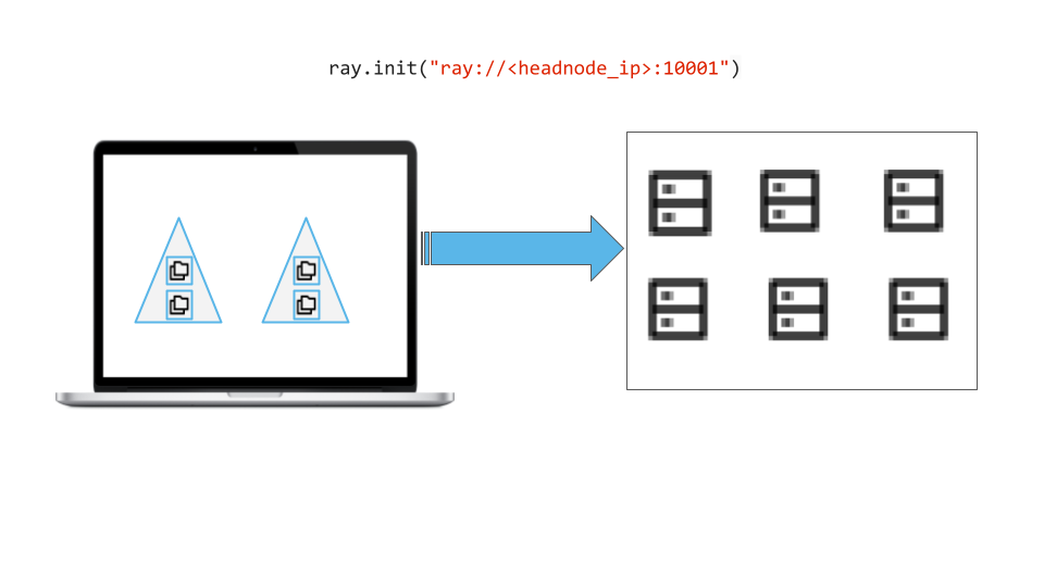Figure 2. The laptop extends or connects to a Ray cluster via a Ray Client

Although opinionated, Ray not only scales your Python applications. It also scales your machine learning workloads. This dual functionality to develop locally on a laptop (with small datasets and limited compute) and then extend remotely to a Ray cluster (with large datasets and elastic compute-resources) is a coveted yet opinionated consideration.

Next, we examine Ray Tune and Ray Train for tuning and training at scale and an open-source ML lifecycle management tool integration with Ray for tracking your ML experiments.

LinkTuning and training at scale and tracking model experiments

As stated in part 1, unlike the traditional software development cycle, the model development cycle paradigm is different. As a result, several factors influence an ML model’s success in production. Of all aspects mentioned in part 1, let’s consider a few and elaborate on them: model tuning, distributed model training, and both model training and tuning together at scale and model experiment tracking. 

Take model tuning at scale. Developing models with state-of-art ML frameworks, such as XGBoost, PyTorch, TensorFlow, or HuggingFace, are compute-intensive ML workloads; they use distributed tuning to reduce total tuning time, employ hyperparameter optimization (HPO) over its search space to obtain the best model parameter configs for best model accuracy, and may need batch inference—all at horizontal scale—from your laptop or a single node with multiple cores to multiple nodes with multiple cores.

For all the above tuning compute-intensive tasks, Ray Tune is most suitable. At its core, Ray Tune leverages cluster resources to scale and distribute trials, each with its hyperparameter configuration and employs proven the state of the art (SOTA) algorithms. For example: 

• Launch a multi-core, single-node, or multi-core, multi-node hyperparameter sweep in a few lines of code

• Use popular ML frameworks such as XGBoost, Scikit-learn, PyTorch, or TensorFlow

• Support state-of-the-art hyperparameter optimization algorithms such as Population Based Training (PBT), HyperBand, or Asynchronous Successive Halving (ASHA)

• Provide cost-saving optimization techniques such as early-stopping, and use of spot instances

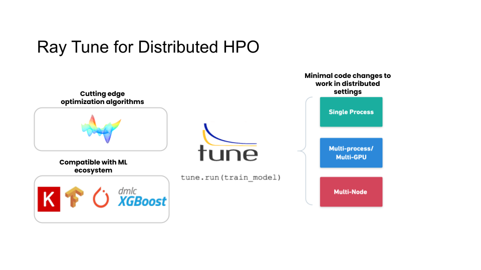Figure 3. Ray Tune for tuning and hyperparameter optimization

By capitalizing on Ray Tune’s above feature functionality and its easy-to-use APIs, you can write tuning trials to run on a single node (multiple cores) or extend and scale it to the cluster with multiple nodes (multiple cores). Three simple steps are all you need in your Python code.

LinkStep 1: Define your objective function for training with Trainable APIs 

1import ray
2from ray import tune
3
4def evaluation_fn(step, width, height):
5    time.sleep(0.1)
6    return (0.1 + width * step / 100)**(-1) + height * 0.1
7
8def easy_objective(config):
9    # fetch our Hyperparameters sent as arguments
10    width, height = config["width"], config["height"]
11    # Iterate over number of steps
12    for step in range(config["steps"]):
13        # Iterative training function - can be any arbitrary training procedure
14        # Here our objective function is the evaluation_fn
15        intermediate_score = evaluation_fn(step, width, height)
16        # Feed the score back back to Tune for each step.
17        tune.report(iterations=step, mean_loss=intermediate_score)

LinkStep 2: Use Ray Tune APIs to execute tuning

1analysis = tune.run(
2    easy_objective,
3    metric="mean_loss",
4    mode="min",
5    num_samples=5,		# number of trials to parallelize 
6    # Define our hyperparameter search space
7    config={
8        "steps": 5,      # this is like number of epochs
9        "width": tune.uniform(0, 20),
10        "height": tune.uniform(-100, 100),
11        "activation": tune.grid_search(["relu", "tanh"]),
12    },
13    verbose=1
14)

LinkStep 3: Analyze the results

1analysis.results_df.head(5)
2analysis.trials
3analysis.dataframe(metric="mean_loss", mode="min").head(5)

You can explore complete code and examples of using Ray Tune to tune and distribute your trials at scale here. All examples follow more or less the same three steps. First, you can execute code on your laptop for experimentation with small datasets—and then extend and scale to the cluster with large datasets. More importantly, these code examples illustrate how to use efficient search algorithms, combined with scheduling algorithms, along with integrations with popular tuning libraries such as Hyperopt and Optuna, giving you the tools and techniques to do model training and tuning at scale. 

In short, if you need to tune your model over a hyperparameter search space and you want to distribute its trials to produce the best config for the best model, use Ray Tune. 

Aside from tuning, let’s consider distributed model training for deep learning. As a lightweight library for distributed deep learning, Ray Train allows you to: 

• Scale your training code from a single node and multiple cores to multiple nodes and multi-cores in a Ray cluster

• Leverage distributed data-parallel deep learning training for PyTorch or TensorFlow models

• Offers composability and interoperability with Ray Tune to tune your distributed model and Ray Datasets to train with large amounts of data 

• Track experiments and training runs with MLflow, using callbacks functions

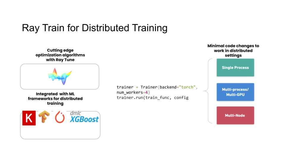Figure 4. Ray Train for distributed deep learning training

As with Ray Tune, so with Ray Train, you can use simple, intuitive APIs and follow three steps to get going: 

LinkStep 1: Define your neural network

In this case, we use PyTorch, but you can just as easily use TensorFlow.

1import torch
2import torch.nn as nn
3import torch.optim as optim
4
5# import from Ray 
6from ray import train
7from ray.train import Trainer
8
9NUM_SAMPLES = 20             # our dataset for training
10INPUT_SIZE = 20              # inputs or neurons into the first layer
11LAYER_SIZE = 15              # inputs or neurons to the hidden layer
12OUTPUT_SIZE = 5              # outputs to the last layer
13
14# In this example we use a randomly generated dataset.
15input = torch.randn(NUM_SAMPLES, INPUT_SIZE)         # In normal ML parlance, X
16labels = torch.randn(NUM_SAMPLES, OUTPUT_SIZE)       # In normal ML parlance, y
17
18class NeuralNetwork(nn.Module):
19    def __init__(self):
20        super(NeuralNetwork, self).__init__()
21        self.layer1 = nn.Linear(in_features=INPUT_SIZE, out_features=LAYER_SIZE)
22        # Our activation function
23        self.relu = nn.ReLU()           
24        self.layer2 = nn.Linear(in_features=LAYER_SIZE, out_features=OUTPUT_SIZE)
25
26    def forward(self, input):
27        return self.layer2(self.relu(self.layer1(input)))

LinkStep 2: Define your training function used by Ray Train

1def train_func_distributed(config):
2
3    model = NeuralNetwork()
4    model = train.torch.prepare_model(model, move_to_device=True)
5    loss_fn = nn.MSELoss()
6    optimizer = optim.SGD(model.parameters(), lr=0.1)
7
8    # Iterate over the loop
9    epochs = config.get('NUM_EPOCHS', [20, 40, 60])
10    for epoch in epochs: 
11        for e in tqdm(range(epoch)):
12            output = model(input)
13            loss = loss_fn(output, labels)
14
15            optimizer.zero_grad()
16            loss.backward()
17            optimizer.step()
18
19            if e % epoch == 0:
20                print(f'epoch {epoch}, loss: {loss.item():.3f}')
21
22    # Return anything you want, here we just report back the PID 
23    # on which this function runs on a remote or local distributed worker process 
24   return os.getpid()

LinkStep 3: Use Ray Train API to distribute training 

We create a Trainer, the main class. This trainer, in turn, will auto-connect to a Ray cluster without the code explicitly calling ray.init(...). If it’s running on a laptop, the trainer will connect to Ray locally, using four worker processes on four cores for distributed training. If the laptop is configured to connect to a cluster, the trainer will extend the laptop, via Ray client, to a remote Ray cluster, using four worker nodes and its cores. As your demands grow, where you need more compute, you can scale num_workers. 

1trainer = Trainer(backend='torch', num_workers=4)
2trainer.start()
3results = trainer.run(train_func_distributed, config={'NUM_EPOCHS': [20, 40, 60]})
4trainer.shutdown()

You can explore complete code and examples using Ray Train for distributed training. All examples follow more or less the same three steps. And your training code can be executed on your laptop for experimentation with small datasets or extended to the cluster for horizontal scaling with large datasets.

Note: Ray Train is still in beta in Ray 1.9 release. However, you can read its rich and extensive feature support in the announcement blog.  

In short, if you need to train your deep learning model using distributed data-parallel with PyTorch or TensorFlow, use Ray Train. But it does not stop you from using both (Ray Tune and Ray Train) when the need arises, as we explain next.

LinkStep 4: Optionally, use Ray Tune with Ray Train API 

Ray Tune is interoperable with Ray Train, and it is natively supported in Ray Train. Such interoperability and composability are desirable design traits among Ray’s native libraries. In some use cases, where you want to have configurable epochs or network architectures, you can use both of these Ray’s native libraries together. 

For brevity, we will skip the code here. Instead, an example guide and steps show how you can convert your Trainer into a Tune trainable—and use it within Ray Tune.

LinkTracking model experiments with MLflow

The last consideration we wish to elaborate on is how to track your experiments and how to examine their results from tuning trials and training runs’ metrics and parameters. Consider the popular open-source machine learning lifecycle management platform MLflow. We recommend it for a few reasons. One is that MLflow supports the most popular ML frameworks’ model flavors. The second is that its APIs are fluent and Pythonic. And third, both Ray Tune and Ray Train have robust integrations with MLflow. 

Whether tuning your models with Ray Tune or distributed training models with Ray Train, you can easily log all your metrics, parameters, and artifacts by providing respective callbacks: MLflowLoggerCallback (for Tune) MLflowLoggerCallback (for Train) in Ray Tune’s and Train’s APIs. For example, to use it with Tune:

1def train_model(config):
2    model = ConvNet(config)
3    for i in range(epochs):
4        current_loss = model.train()
5    tune.report(loss=current_loss)
6 …
7
8tune.run(
9    train_model,
10    config={“lr”: tune.uniform(0.001, 0.1)},
11    num_samples=100,
12    callbacks=[MLflowLoggerCallback(“my_experiment”)])

This callback interacts with the MLflow Tracking Server and logs all its metrics, parameters, and artifacts under an MLflow experiment name “my_experiment.”

Similarly, with Ray Train, you too can provide a callback to log all metrics, parameters, or artifacts reported back to the train driver from the distributed trainers and logged by the train driver. You can peruse a complete code example, in its entirety, for distributed training on big data at scale using MLflow here. 

Finally, all the results logged to the MLflow Tracking Server can be viewed in the MLflow UI.

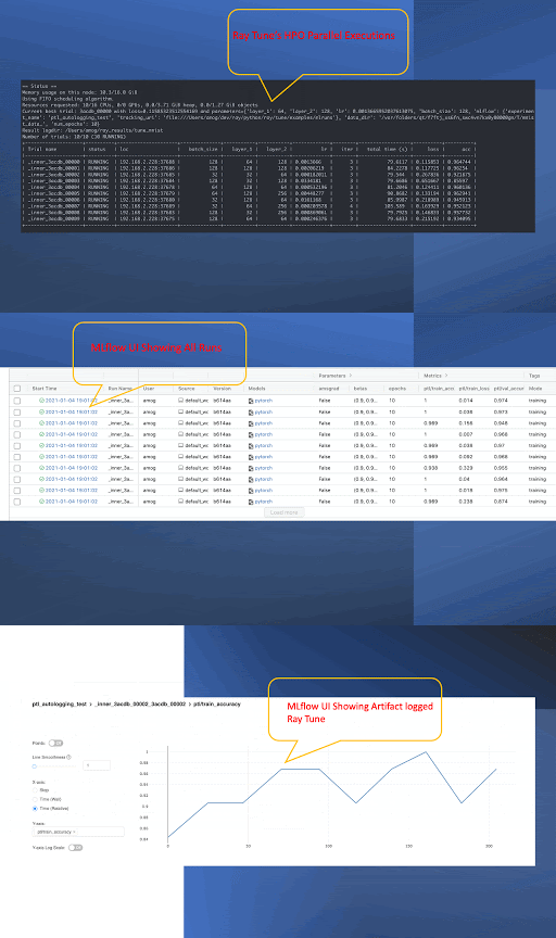Figure 5: MLflow Integrations: Ray Tune & Train

Altogether, using a laptop for developing and extending to a Ray cluster, model tuning and distributed training at scale using Ray Tune and Ray Train, and instrumenting and tracking the results of all your trials and training runs with MLflow are vital considerations as part of ML model’s journey to production. 

LinkConclusion

Let’s recap. In this second part, we elaborated and opinionated on two considerations for ML in production: 1) developing with ease and 2) tuning and training at scale and tracking model experiments. For the first, we shared methods how developers can replicate and isolate their staging or production environments—for Python dependencies—on their laptops using conda environments; how they can then build and test their ML models, using popular ML frameworks of their choice, with small datasets and then easily extend to a Ray cluster. 

As for the second, we elaborated how Ray Tune, Ray Train, and their respective MLflow integrations help you scale and distribute your model training, tuning, and tracking on your laptop and a Ray cluster. In both these considerations, we suggested starting with your laptop first using Ray and its ecosystem and then extending to a Ray cluster to scale your ML applications in production. One satisfied Ray ML engineer and blogger wrote:

Today, no one doubts that we have come a long way from the 1949 British newspaper’s pessimistic lament of the unrealized power of computers. Today’s powerful laptops offer the best integrated, developer-friendly, and productive environments. And their effortless ability to extend (or connect) to the cluster is as normal as taking a daily-commuter flight and using WiFi at 30,000 feet. No speculation, just a fact.

In the final blog in this series, we will examine consideration #4: deploying, serving, and inferencing models at scale.