In reinforcement learning (RL), like in supervised learning (SL), we use neural network (NN) models as trainable function approximators. The inputs to these models are observation tensors from the environment that we would like to master (e.g. a simulation, a game, or a real-world scenario), and our network then computes actions to execute in this environment. The goal of any RL algorithm is to train the neural network, such that its action choices become optimal with respect to a reward signal, which is also provided by the environment. We often refer to our neural network function as the policy or π:
action = π(observation) (Eq. 1)

In the common case above (Eq. 1), observation is the current “frame” seen by the agent, but more and more often we’re seeing RLlib users try out models where this isn’t enough. For example:

• In “frame stacking”, the model sees the last n observations to account for the fact that a single time frame does not capture the entire state of the environment (think of a ball seen in a screenshot of a game and we wouldn’t know whether it’s flying to the left or right).

  action = π(observations[t, t-1, t-2, ..]) (Eq. 2)

• In recurrent neural networks (RNN), the model sees the last observation, but also a tracked hidden state or memory vector that has previously been produced by that model itself and is altered over time:

  action, memory[t] = π(observation[t], memory[t-1]). (Eq. 3)

• Furthermore, in attention nets (e.g. transformer models), the model sees the last observation and also the last N tracked memory vectors:

  action, memory[t] = π(observation[t], memory[t-n:t]) (Eq. 4)

In this blog post, we’ll cover RLlib’s new trajectory view API that makes these complex policy models possible (and fast). Building on that functionality, we’ll show how this enables efficient attention net support in RLlib.

LinkThe Trajectory View API

The trajectory view API should solve two major problems: a) Make complex model support possible and — along with that — b) allow for a faster (environment) sample collection and retrieval system.

The trajectory view API is a dictionary, mapping keys (str) to “view requirement” objects. The defined keys correspond to available keys in the input-dicts (or SampleBatches) with which our models are called. We also call these keys “views”. The dict is defined in a models’ constructor (see the self.view_requirements property of the ModelV2 class). In the default case, it contains only one entry (the “obs” key). The value is a ViewRequirement object telling RLlib to not perform any “shifts” (time-wise) on the collected observations for this view:

self.view_requirements = {“obs”: ViewRequirement(shift=0)}

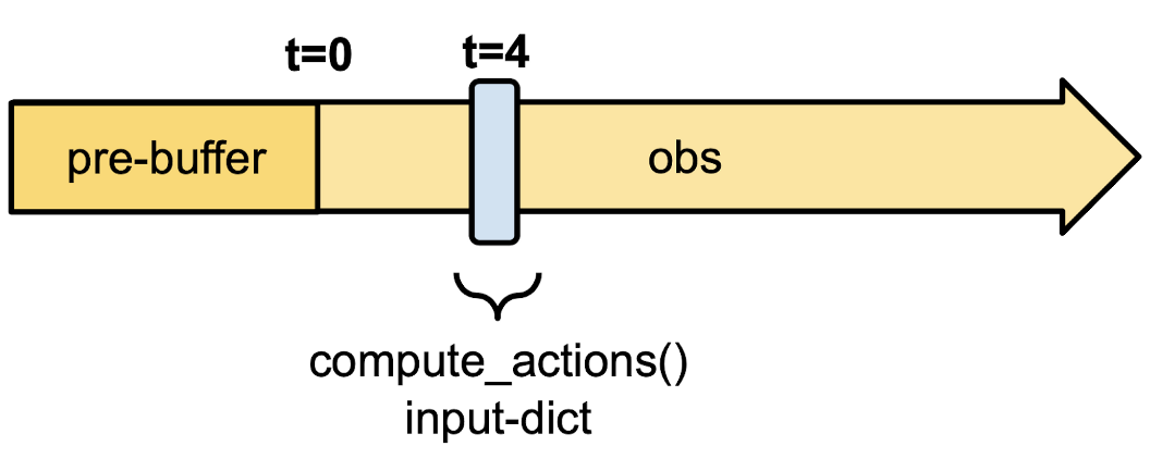Figure 1: Default view requirements and the effect of this setup on the internal data storage. The pre-buffer exists for possible negative shifts requiring to zero-initialize time steps before the actual start of the episode (see Fig. 2 and the frame stacking case for more information).

Here, the model tells us that it needs the current observation as input (e.g. for calculating the 4th action in an episode, it requires the 4th observation; Fig. 1).

Let’s take a look at the “frame stacking” case. Frame stacking is done to add some sense of time to the model’s input by stacking up the last n observations (as is commonly done for example in Atari experiments) and treating the resulting tensor as one:

self.view_requirements = {“obs”: ViewRequirement(shift=[-3, -2, -1, 0])}

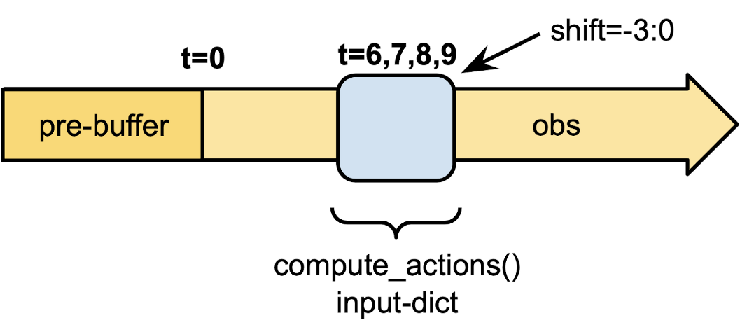Figure 2: An example for a frame-stacking setup. RLlib will provide the last 4 observations (t-3 to t=0) to the model in each forward pass. Here, we show the input at time step t=9. Alternatively, for the shift argument, we can also use the string: "-3:0". Note here that the last shift index (0) will be included in the generated view.

We can now see more easily why a better and more efficient sample storage and retrieval system was needed to implement the trajectory view API: The pre-buffer in Fig. 2 helps in case past information from the episodes is required at t=0. For example, to compute an action at time step 0, no previous observations exist and RLlib will provide zero-filled dummy values (from the pre-buffer) for frames -3, -2, and -1 (Fig. 2). More importantly, instead of storing an [n x O] sized tensor where n=stacking size (n=4 in Fig. 2) and O=observation size at each single(!) timestep, like we used to do before the trajectory view API was introduced, we can now reduce the memory complexity by a factor of `s`.

The new storage and retrieval API is defined by the SampleCollector class and its default implementation is a simple list-based collector. You can implement your own collection- and storage mechanisms, such as e.g. the method proposed in the “Sample Factory” paper. However, RLlib’s default SampleCollector (a simple, list-based collector) is already helping to make the algorithms considerably faster (Table 1) compared to the previous collection- and storage solutions.

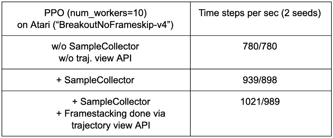Table 1: Top row: Classic performance (no SampleCollector, no trajectory view API-based frame stacking); Middle row: A speedup of ~15–20% was achieved for PPO by more cleverly collecting and storing samples from an Atari ("BreakoutNoFrameskip-v4") environment. Bottom row: When also using the trajectory view API to handle the 4x frame stacking (see Fig. 2), an additional 10% speedup can be observed.

RLlib’s built-in LSTMs have yet more complex view requirements, as they also require previous memory outputs and possibly previous actions and/or rewards as inputs (besides the observations). For example:

1self.view_requirements = {
2
3    "obs": ViewRequirement(shift=[-3, -2, -1, 0]),
4
5    "state_in_0": ViewRequirement(data_col="state_out_0", shift=-1),
6
7    "prev_actions": ViewRequirement(data_col="actions", shift=-1),
8
9}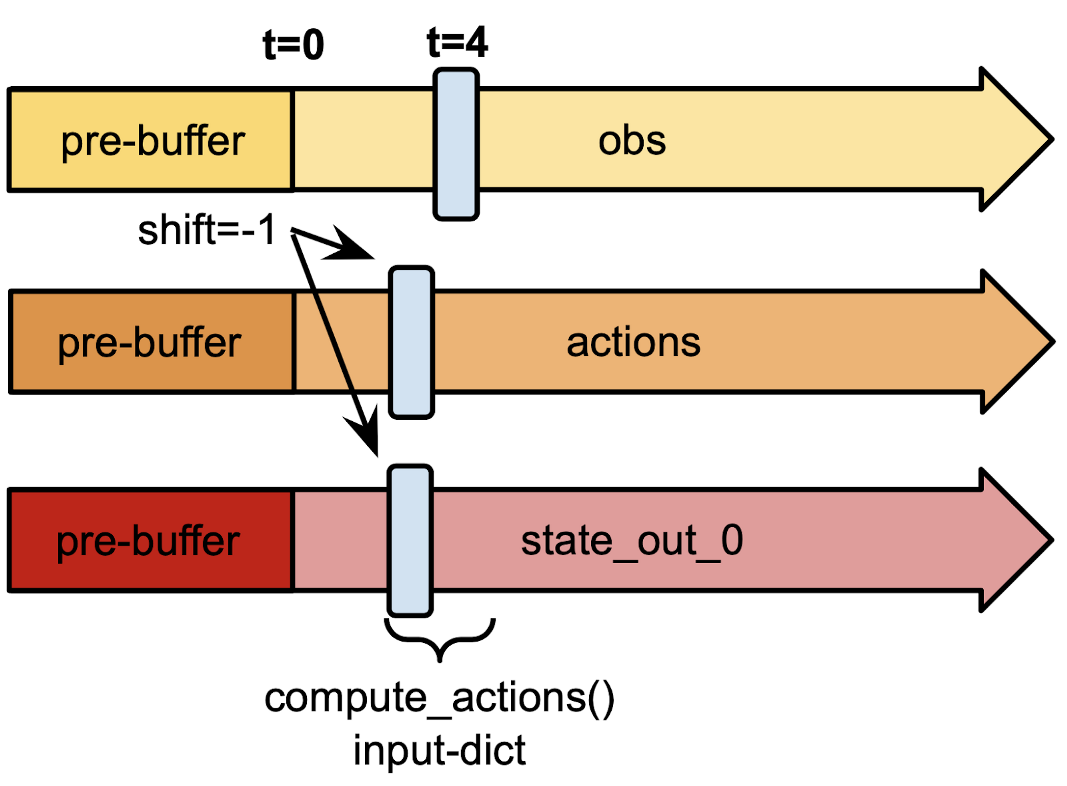

Figure 3: An RNN model asking for the current observation, the previous action and the previous memory (state) output. Note that both actions and memory (state) are actually produced by the model itself. Also, if we are at t=0, the previous action and memory will be taken from the (zero-initialized) pre-buffer.

Note that the “state_in_0” view in Fig. 3 relies on previous “state_out_0” outputs and thus saves further memory (prior to the trajectory view API, we would store state-ins and state-outs separately and therefore requiring twice the space). Similarly, the “prev_actions” view relies on previous “actions” outputs (also no extra memory required).

In the next section, we will talk about attention nets and their particular view requirements setup.

LinkAttention Nets in RLlib

For our new built-in attention net implementations (based on the GTrXL paper here), we are using a trajectory view setup like this:

1self.view_requirements = {
2
3    "obs": ViewRequirement(shift=[-3, -2, -1, 0]),
4
5    "state_in_0": ViewRequirement(data_col="state_out_0",
6        shift="-50:-1"),
7
8}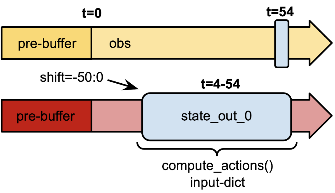

Figure 4: An attention net (e.g. RLlib's GTrXLs) needs to "see" the previous n (here: 50) memory outputs (state_out_0). Compared to a previous implementation of GTrXL, the trajectory view API and SampleCollector mechanism now allows us to reduce the memory complexity by 2 x n (2 b/c we only store state-outs, not state-ins; n b/c we only store each timestep's single state-out tensor).

This allows us to a) only store the state-out tensors (no need for storing state-ins separately), as well as b) to store only a single memory tensor per timestep as opposed to a previous RLlib GTrXL implementation, where we had to store n-stacked tensors per single timestep(!). Thus, in total, this reduces the required memory by 2 x n (where n is the stacking value; 50 in the above example).

LinkPutting it all together: Stateless Cartpole example

“CartPole” is a popular environment provided by the openAI gym to quickly test the learning capabilities of an RL algorithm. Its observations are vectors of dim=4, containing the x-position, x-velocity, the angle of the pole, and the angular velocity of the pole (see Figure 5).

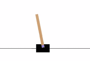Figure 5: CartPole-v0, a popular openAI gym environment to quickly test and debug RL agents, can be transformed into a PO-MDP (partially observable MDP) by removing the angular- and spatial velocity values from the observation tensors.

Now imagine we take away the x-velocity and angular velocity inputs from the observation vector and thereby make this environment a partially observable one (i.e. we can no longer know what the x-velocity is, given we only have the current x-position). We call this environment “stateless” CartPole and it is unsolvable by vanilla PPO or DQN algos. To solve “stateless” CartPole, we will setup a quick frame-stacking solution in RLlib (and even stack past actions and past rewards), using the trajectory view API. By taking a quick look at our PyTorch model, we can see that in its constructor, the view requirements are defined as follows:

1self.view_requirements["prev_n_obs"] = ViewRequirement(
2
3    data_col="obs",
4
5    shift="-{}:0".format(num_frames - 1),
6
7    space=obs_space)
8
9self.view_requirements["prev_n_rewards"] = ViewRequirement(
10
11    data_col="rewards", shift="-{}:-1".format(self.num_frames))
12
13self.view_requirements["prev_n_actions"] = ViewRequirement(
14
15    data_col="actions",
16
17    shift="-{}:-1".format(self.num_frames),
18
19    space=self.action_space)

.. where num_frames is the number of frames we would like to look back. Note that we can now access the defined “views” (e.g. “prev_n_actions”) inside our model via the input-dict that is always passed in. By setting these three keys in the view_requirements dict, we are telling RLlib to present not just the current observation, but the last n observations, the last n actions, and the last n rewards to our model’s forward call.

We then run a quick experiment using the code in this example script here:

1import ray
2
3from ray import tune
4
5from ray.rllib.examples.env.stateless_cartpole import StatelessCartPole
6
7from ray.rllib.examples.models.trajectory_view_utilizing_models import TorchFrameStackingCartPoleModel
8
9from ray.rllib.models.catalog import ModelCatalog
10
11ModelCatalog.register_custom_model("frame_stack_model", TorchFrameStackingCartPoleModel)
12
13tune.register_env("stateless_cartpole", lambda c: StatelessCartPole())
14
15ray.init()
16
17tune.run("PPO", config={
18
19    "env": "stateless_cartpole",
20
21    "model": {
22
23        "custom_model": "frame_stack_model",
24
25        "custom_model_config": {
26
27            "num_frames": 16,
28        }
29    },
30
31    "framework": "torch",
32
33})

We now compare the above model with a) using an LSTM- and b) using an attention-based model. For all three experiments (frame-stacking model, LSTM, attention), we setup a 2x256 dense core network and RLlib’s default PPO config (with 3 minor changes described in the table below).

Table 2: Timesteps needed to solve the stateless CartPole environment (CartPole-v0, but w/o emitting x-velocity or angular velocity values) with RLlib's PPO on 2 rollout workers, up to a mean episode reward of 150.0. LSTM- and attention models were fed only the last action and reward, whereas the frame-stacking model received the last 16 observations, actions and rewards. All models had a 2x256 dense layer "core".

LinkWhat’s next?

To recap, we covered a new RLlib API for complex policy models, and showed how this enables efficient sample collection and retrieval. In a future blog post, we will be focusing on attention nets (one of the big winners, performance-wise, of the trajectory view API efforts) and how they can be used in RLlib to solve much more complex, visual navigation environments, such as VizDoom-, Unity’s Obstacle Tower, or the DeepMind Lab environments.

If you would like to see how RLlib is being used in industry, you should check out Ray Summit for more information. Also, consider joining the Ray discussion forum. It’s a great place to ask questions, get help from the community, and — of course — help others as well.