[ GitHub |  Notebook | Anyscale Endpoints | Ray Docs]  · 45 min read

In this guide, we will learn how to:

• 💻 Develop a retrieval augmented generation (RAG) based LLM application from scratch.

• 🚀 Scale the major workloads (load, chunk, embed, index, serve, etc.) across multiple workers.

• ✅ Evaluate different configurations of our application to optimize for both per-component (ex. retrieval_score) and overall performance (quality_score).

• 🔀 Implement LLM hybrid routing approach to bridge the gap b/w OSS and closed LLMs.

• 📦 Serve the application in a highly scalable and available manner.

• 💥 Share the 1st order and 2nd order impacts LLM applications have had on our products.

LinkOverview

Large language models (LLMs) have undoubtedly changed the way we interact with information. However, they come with their fair share of limitations as to what we can ask of them. Base LLMs (ex. Llama-2-70b, gpt-4, etc.) are only aware of the information that they've been trained on and will fall short when we require them to know information beyond that. Retrieval augmented generation (RAG) based LLM applications address this exact issue and extend the utility of LLMs and their generative reasoning abilities to our unique datasets. 

In this guide, we're going to build a RAG-based LLM application where we will incorporate external data sources to augment our LLM’s capabilities. Specifically, we will be building an assistant that can answer questions about Ray — a Python framework for productionizing and scaling ML workloads. The goal here is to make it easier for developers to adopt Ray, but also, as we'll see in this guide, to help improve our Ray documentation itself and provide a foundation for other LLM applications. We’ll also share challenges we faced along the way and how we overcame them.

Note: We have generalized this entire guide so that it can easily be extended to build RAG-based LLM applications on top of your own data.

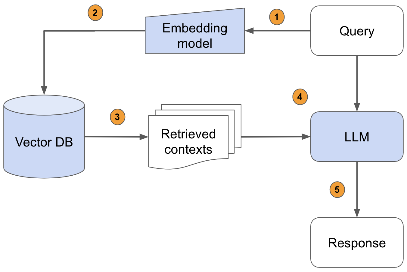
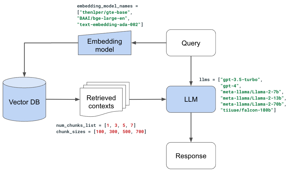
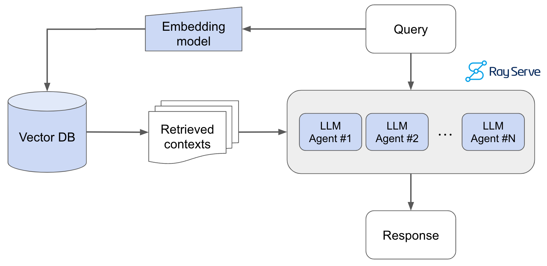
1. Pass the query to the embedding model to semantically represent it as an embedded query vector.

2. Pass the embedded query vector to our vector DB.

3. Retrieve the top-k relevant contexts – measured by distance between the query embedding and all the embedded chunks in our knowledge base.

4. Pass the query text and retrieved context text to our LLM.

5. The LLM will generate a response using the provided content.

Besides just building our LLM application, we’re also going to be focused on scaling and serving it in production. Unlike traditional machine learning, or even supervised deep learning, scale is a bottleneck for LLM applications from the very beginning. Large datasets, models, compute intensive workloads, serving requirements, etc. We’ll develop our application to be able to handle any scale as the world around us continues to grow.

We’re also going to be focused on evaluation and performance. Our application involves many moving pieces: embedding models, chunking logic, the LLM itself, etc. and so it's important that we experiment with different configurations to optimize for the best quality responses. However, it's non-trivial to evaluate and quantitatively compare different configurations for a generative task. We’re going to break down evaluation of individual parts of our application (retrieval given query, generation given source), also assess the overall performance (end-to-end generation) and share findings towards an optimized configuration.

Note: We'll be experimenting with different LLMs (OpenAI, Llama, etc.) in this guide. You will need OpenAI credentials to access ChatGPT models and Anyscale Endpoints (public and private endpoints available) to access + fine-tune OSS LLMs.

LinkDatabase Creation

Before we can start building our RAG application, we need to first create our vector DB that will contain our processed data sources.

LinkLoad data

We’re going to start by loading the Ray documentation from the website to a local directory:

1export EFS_DIR=/desired/output/directory
2wget -e robots=off --recursive --no-clobber --page-requisites \
3  --html-extension --convert-links --restrict-file-names=windows \
4  --domains docs.ray.io --no-parent --accept=html \
5  -P $EFS_DIR https://docs.ray.io/en/master/

We’re going to then load our docs contents into a Ray Dataset so that we can perform operations at scale on them (ex. embed, index, etc.). With large data sources, models and application serving needs, scale is a day-1 priority for LLM applications. We want to build our applications in such a way that they can scale as our needs grow without us having to change our code later.

1# Ray dataset
2DOCS_DIR = Path(EFS_DIR, "docs.ray.io/en/master/")
3ds = ray.data.from_items([{"path": path} for path in DOCS_DIR.rglob("*.html") 
4if not path.is_dir()])
5print(f"{ds.count()} documents")

LinkSections

Now that we have a dataset of all the paths to the html files, we're going to develop some functions that can appropriately extract the content from these files. We want to do this in a generalized manner so that we can perform this extraction across all of our docs pages (and so you can use it for your own data sources). Our process is to first identify the sections in our html page and then extract the text in between them. We save all of this into a list of dictionaries that map the text within a section to a specific url with a section anchor id.

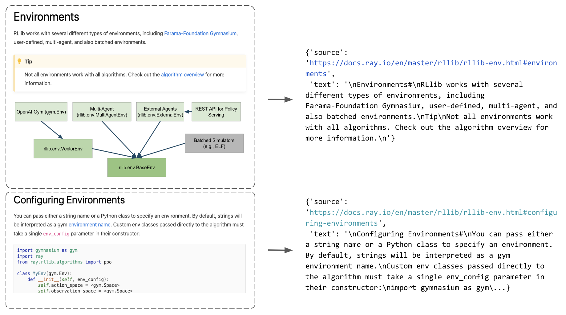
1sample_html_fp = Path(EFS_DIR, "docs.ray.io/en/master/rllib/rllib-env.html")
2extract_sections({"path": sample_html_fp})[0]
3

{'source': 'https://docs.ray.io/en/master/rllib/rllib-env.html#environments', 'text': '\nEnvironments#\nRLlib works with several different types of environments, including Farama-Foundation Gymnasium, user-defined, multi-agent, and also batched environments.\nTip\nNot all environments work with all algorithms. Check out the algorithm overview for more information.\n'}

We can apply this extraction process (extract_section) in parallel to all the file paths in our dataset with just one line using Ray Data’s flat_map.

1# Extract sections
2sections_ds = ds.flat_map(extract_sections)
3sections = sections_ds.take_all()
4print (len(sections))
5

LinkChunk data

We now have a list of sections (with text and source of each section) but we shouldn't directly use this as context to our RAG application just yet. The text lengths of each section are all varied and many are quite large chunks. 

If we were to use these large sections, then we'd be inserting a lot of noisy/unwanted context and because all LLMs have a maximum context length, we wouldn't be able to fit too much other relevant context. So instead, we're going to split the text within each section into smaller chunks. Intuitively, smaller chunks will encapsulate single/few concepts and will be less noisy compared to larger chunks. We're going to choose some typical text splitting values (ex. chunk_size=300) to create our chunks for now but we'll be experimenting with a wider range of values later.

1from langchain.document_loaders import ReadTheDocsLoader
2from langchain.text_splitter import RecursiveCharacterTextSplitter
3
4# Text splitter
5chunk_size = 300
6chunk_overlap = 50
7text_splitter = RecursiveCharacterTextSplitter(
8    separators=["\n\n", "\n", " ", ""],
9    chunk_size=chunk_size,
10    chunk_overlap=chunk_overlap,
11    length_function=len,
12)
13
14# Chunk a sample section
15sample_section = sections_ds.take(1)[0]
16chunks = text_splitter.create_documents(
17    texts=[sample_section["text"]], 
18    metadatas=[{"source": sample_section["source"]}])
19print (chunks[0])
20

page_content='ray.tune.TuneConfig.search_alg#\nTuneConfig.search_alg: Optional[Union[ray.tune.search.searcher.Searcher, ray.tune.search.search_algorithm.SearchAlgorithm]] = None#' metadata={'source': 'https://docs.ray.io/en/master/tune/api/doc/ray.tune.TuneConfig.search_alg.html#ray-tune-tuneconfig-search-alg'}

While chunking our dataset is relatively fast, let’s wrap the chunking logic into a function so that we can apply the workload at scale so that chunking remains just as fast as our data sources grow:

1def chunk_section(section, chunk_size, chunk_overlap):
2    text_splitter = RecursiveCharacterTextSplitter(
3        separators=["\n\n", "\n", " ", ""],
4        chunk_size=chunk_size,
5        chunk_overlap=chunk_overlap,
6        length_function=len)
7    chunks = text_splitter.create_documents(
8        texts=[sample_section["text"]], 
9        metadatas=[{"source": sample_section["source"]}])
10    return [{"text": chunk.page_content, "source": chunk.metadata["source"]} for chunk in chunks]
11
12# Scale chunking
13chunks_ds = sections_ds.flat_map(partial(
14    chunk_section, 
15    chunk_size=chunk_size, 
16    chunk_overlap=chunk_overlap))
17print(f"{chunks_ds.count()} chunks")
18chunks_ds.show(1)
19

5727 chunks
{'text': 'ray.tune.TuneConfig.search_alg#\nTuneConfig.search_alg: Optional[Union[ray.tune.search.searcher.Searcher, ray.tune.search.search_algorithm.SearchAlgorithm]] = None#', 'source': 'https://docs.ray.io/en/master/tune/api/doc/ray.tune.TuneConfig.search_alg.html#ray-tune-tuneconfig-search-alg'}

LinkEmbed data

Now that we've created small chunks from our sections, we need a way to identify the most relevant ones for a given query. A very effective and quick method is to embed our data using a pretrained model and use the same model to embed the query. We can then compute the distance between all of the chunk embeddings and our query embedding to determine the top-k chunks. There are many different pretrained models to choose from to embed our data but the most popular ones can be discovered through HuggingFace's Massive Text Embedding Benchmark (MTEB) leaderboard. These models were pretrained on very large text corpus through tasks such as next/masked token prediction which allowed them to learn to represent sub-tokens in N dimensions and capture semantic relationships. We can leverage this to represent our data and identify the most relevant contexts to use to answer a given query. We're using Langchain's Embedding wrappers (HuggingFaceEmbeddings and OpenAIEmbeddings) to easily load the models and embed our document chunks.

Note: embeddings aren't the only way to determine the more relevant chunks. We could also use an LLM to decide! However, because LLMs are much larger than these embedding models and have maximum context lengths, it's better to use embeddings to retrieve the top k chunks. And then we could use LLMs on the fewer k chunks to determine the <k chunks to use as the context to answer our query. We could also use reranking (ex. Cohere Rerank) to further identify the most relevant chunks to use. We could also combine embeddings with traditional information retrieval methods such as keyword matching, which could be useful for matching for unique tokens that may potentially be lost when embedding sub-tokens.

1from langchain.embeddings import OpenAIEmbeddings
2from langchain.embeddings.huggingface import HuggingFaceEmbeddings
3import numpy as np
4from ray.data import ActorPoolStrategy
5
6class EmbedChunks:
7    def __init__(self, model_name):
8        if model_name == "text-embedding-ada-002":
9            self.embedding_model = OpenAIEmbeddings(
10                model=model_name,
11                openai_api_base=os.environ["OPENAI_API_BASE"],
12                openai_api_key=os.environ["OPENAI_API_KEY"])
13        else:
14            self.embedding_model = HuggingFaceEmbeddings(
15                model_name=model_name,
16                model_kwargs={"device": "cuda"},
17                encode_kwargs={"device": "cuda", "batch_size": 100})
18
19    def __call__(self, batch):
20        embeddings = self.embedding_model.embed_documents(batch["text"])
21        return {"text": batch["text"], "source": batch["source"], "embeddings": 
22embeddings}
23

Here we're able to embed our chunks at scale by using map_batches. All we had to do was define the batch_size and the compute (we're using two workers, each with 1 GPU).

1# Embed chunks
2embedding_model_name = "thenlper/gte-base"
3embedded_chunks = chunks_ds.map_batches(
4    EmbedChunks,
5    fn_constructor_kwargs={"model_name": embedding_model_name},
6    batch_size=100, 
7    num_gpus=1,
8    compute=ActorPoolStrategy(size=2))
9

# Sample (text, source, embedding) triplet
[{'text': 'External library integrations for Ray Tune#',
  'source': 'https://docs.ray.io/en/master/tune/api/integration.html#external-library-integrations-for-ray-tune',
  'embeddings': [
0.012108353897929192,
0.009078810922801495,
0.030281754210591316,
-0.0029687234200537205,
…]
}

LinkIndex data

Now that we have our embedded chunks, we need to index (store) them somewhere so that we can retrieve them quickly for inference. While there are many popular vector database options, we're going to use Postgres with pgvector for its simplicity and performance. We'll create a table (document) and write the (text, source, embedding) triplets for each embedded chunk we have.

1class StoreResults:
2    def __call__(self, batch):
3        with psycopg.connect(os.environ["DB_CONNECTION_STRING"]) as conn:
4            register_vector(conn)
5            with conn.cursor() as cur:
6                for text, source, embedding in zip
7                (batch["text"], batch["source"], batch["embeddings"]):
8                    cur.execute("INSERT INTO document (text, source, embedding) 
9                    VALUES (%s, %s, %s)", (text, source, embedding,),)
10        return {}
11

And once again, we can use Ray Data’s map_batches to perform this indexing in parallel:

1# Index data
2embedded_chunks.map_batches(
3    StoreResults,
4    batch_size=128,
5    num_cpus=1,
6    compute=ActorPoolStrategy(size=28),
7).count()
8

LinkRetrieval

With our embedded chunks indexed in our vector database, we're ready to perform retrieval for a given query. We'll start by using the same embedding model we used to embed our text chunks to now embed the incoming query.

1# Embed query
2embedding_model = HuggingFaceEmbeddings(model_name=embedding_model_name)
3query = "What is the default batch size for map_batches?"
4
5embedding = np.array(embedding_model.embed_query(query))
6len(embedding)
7

768

Then, we'll retrieve the top-k most relevant chunks by extracting the closest embedded chunks to our embedded query. We use cosine distance (<=>) but there are many options to choose from. Once we retrieve the top num_chunks, we can collect the text for each chunk and use it as context to generate a response.

1# Get context
2num_chunks = 5
3with psycopg.connect(os.environ["DB_CONNECTION_STRING"]) as conn:
4    register_vector(conn)
5    with conn.cursor() as cur:
6        cur.execute("SELECT * FROM document ORDER BY embedding <-> %s LIMIT %s", (embedding, num_chunks))
7        rows = cur.fetchall()
8        context = [{"text": row[1]} for row in rows]
9        sources = [row[2] for row in rows]
10

https://docs.ray.io/en/master/data/api/doc/ray.data.Dataset.map_batches.html#ray-data-dataset-map-batchesentire blocks as batches (blocks may contain different numbers of rows).
The actual size of the batch provided to fn may be smaller than
batch_size if batch_size doesn’t evenly divide the block(s) sent
to a given map task. Default batch_size is 4096 with “default”.

https://docs.ray.io/en/master/data/api/doc/ray.data.Dataset.map_batches.html#ray-data-dataset-map-batches
entire blocks as batches (blocks may contain different numbers of rows).
The actual size of the batch provided to fn may be smaller than
batch_size if batch_size doesn’t evenly divide the block(s) sent
to a given map task. Default batch_size is 4096 with “default”.

(cont…)

LinkGeneration

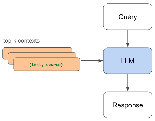
We can now use the context to generate a response from our LLM. Without this relevant context that we retrieved, the LLM may not have been able to accurately answer our question. And as our data grows, we can just as easily embed and index any new data and be able to retrieve it to answer questions.

1from rag.generate import prepare_response
2from rag.utils import get_client
3
4def generate_response(
5    llm, temperature=0.0, stream=True,
6    system_content="", assistant_content="", user_content="", 
7    max_retries=1, retry_interval=60):
8    """Generate response from an LLM."""
9    retry_count = 0
10    client = get_client(llm=llm)
11    messages = [{"role": role, "content": content} for role, content in [
12        ("system", system_content), 
13        ("assistant", assistant_content), 
14        ("user", user_content)] if content]
15    while retry_count <= max_retries:
16        try:
17            chat_completion = client.chat.completions.create(
18                model=llm,
19                temperature=temperature,
20                stream=stream,
21                messages=messages,
22            )
23            return prepare_response(chat_completion, stream=stream)
24
25        except Exception as e:
26            print(f"Exception: {e}")
27            time.sleep(retry_interval)  # default is per-minute rate limits
28            retry_count += 1
29    return ""

Note: We’re using a temperature of 0.0 to enable reproducible experiments but you should adjust this based on your use case. For use cases that need to always be factually grounded, we recommend very low temperature values while more creative tasks can benefit from higher temperatures.

1# Generate response
2query = "What is the default batch size for map_batches?"
3response = generate_response(
4    llm="meta-llama/Llama-2-70b-chat-hf",
5    temperature=0.0,
6    stream=True,
7    system_content="Answer the query using the context provided. Be succinct.",
8    user_content=f"query: {query}, context: {context}")
9

The default batch size for map_batches is 4096.

LinkAgent

Let's combine the context retrieval and response generation together into a convenient query agent that we can use to easily generate our responses. This will take care of setting up our agent (embedding and LLM model), as well as the context retrieval, and pass it to our LLM for response generation.

1class QueryAgent:
2    def __init__(self, embedding_model_name="thenlper/gte-base",
3                 llm="meta-llama/Llama-2-70b-chat-hf", temperature=0.0, 
4                 max_context_length=4096, system_content="", assistant_content=""):
5
6        # Embedding model
7        self.embedding_model = get_embedding_model(
8            embedding_model_name=embedding_model_name, 
9            model_kwargs={"device": "cuda"}, 
10            encode_kwargs={"device": "cuda", "batch_size": 100})
11
12	 # Context length (restrict input length to 50% of total length)
13        max_context_length = int(0.5*max_context_length)
14
15        # LLM
16        self.llm = llm
17        self.temperature = temperature
18        self.context_length =  max_context_length - get_num_tokens(system_content + assistant_content)
19        self.system_content = system_content
20        self.assistant_content = assistant_content
21
22    def __call__(self, query, num_chunks=5, stream=True):
23        # Get sources and context
24        context_results = semantic_search(
25            query=query, 
26            embedding_model=self.embedding_model, 
27            k=num_chunks)
28
29        # Generate response
30        context = [item["text"] for item in context_results]
31        sources = [item["source"] for item in context_results]
32        user_content = f"query: {query}, context: {context}"
33
34        answer = generate_response(
35            llm=self.llm,
36            temperature=self.temperature,
37            stream=stream,
38            system_content=self.system_content,
39            assistant_content=self.assistant_content,
40            user_content=trim(user_content, self.context_length))
41
42        # Result
43        result = {
44            "question": query,
45            "sources": sources,
46            "answer": answer,
47            "llm": self.llm,
48        }
49        return result

With this, we can use our RAG application in just a few lines:

1llm = "meta-llama/Llama-2-7b-chat-hf"
2agent = QueryAgent(
3    embedding_model_name="thenlper/gte-base",
4    llm=llm,
5    max_context_length=MAX_CONTEXT_LENGTHS[llm],
6    system_content="Answer the query using the context provided. Be succinct.")
7result = agent(query="What is the default batch size for map_batches?")
8print("\n\n", json.dumps(result, indent=2))

The default batch size for `map_batches` is 4096

{
  "question": "What is the default batch size for map_batches?",
  "sources": [
"https://docs.ray.io/en/master/data/api/doc/ray.data.Dataset.map_batches.html#ray-data-dataset-map-batches",
"https://docs.ray.io/en/master/data/transforming-data.html#configuring-batch-size",
"https://docs.ray.io/en/master/data/data-internals.html#execution-memory",
"https://docs.ray.io/en/master/serve/advanced-guides/dyn-req-batch.html#tips-for-fine-tuning-batching-parameters", "https://docs.ray.io/en/master/data/examples/pytorch_resnet_batch_prediction.html#model-inference"
  ],
  "answer": "The default batch size for `map_batches` is 4096",
  "llm": "meta-llama/Llama-2-7b-chat-hf"
}

LinkEvaluation

So far, we've chosen typical/arbitrary values for the various parts of our RAG application. But if we were to change something, such as our chunking logic, embedding model, LLM, etc. how can we know that we have a better configuration than before? A generative task like this is very difficult to quantitatively assess and so we need to develop reliable ways to do so.

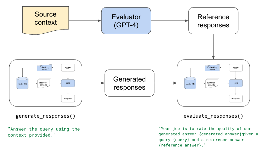
Because we have many moving parts in our application, we need to perform both unit/component and end-to-end evaluation. Component-wise evaluation can involve evaluating our retrieval in isolation (is the best source in our set of retrieved chunks) and evaluating our LLMs response (given the best source, is the LLM able to produce a quality answer). And for end-to-end evaluation, we can assess the quality of the entire system (given the data sources, what is the quality of the response).

We'll be asking our evaluator LLM to score the quality of the response between 1-5 using the context, however, we could also have it produce scores for other dimensions such as hallucination (is the generated answer using information only from the provided context), toxicity, etc.

Note: We could have constrained the score to be binary (0/1), which might be more interpretable (ex. the response was either correct or incorrect). However, we introduced a higher variance in our scores to develop a deeper, fine-grained, understanding of how LLMs score responses (ex. LLM bias towards responses).

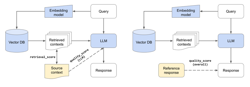
Component evaluations (left) of retrieval system and LLM. Overall evaluation (right).

LinkEvaluator

We're going to start by determining our evaluator. Given a response to a query and relevant context, our evaluator should be a trusted way to score/assess the quality of the response. But before we can determine our evaluator, we need a dataset of questions and the source where the answer comes from. We can use this dataset to ask our different evaluators to provide an answer and then rate their answer (ex. score between 1-5). We can then inspect this dataset to determine if our evaluator is unbiased and has sound reasoning for the scores that are assigned.

Note: We’re evaluating the ability of our LLM to generate a response given the relevant context. This is a component-level evaluation (quality_score (LLM)) because we aren’t using retrieval to fetch the relevant context.

We'll start by manually creating our dataset (keep reading if you can’t manually create a dataset). We have a list of user queries and the ideal source to answer the query datasets/eval-dataset-v1.jsonl. We will use our LLM app above to generate reference answers for each query/source pair using gpt-4.

1with open(Path(ROOT_DIR, "datasets/eval-dataset-v1.jsonl"), "r") as f:
2    data = [json.loads(item) for item in list(f)]
3

[{'question': 'I’m struggling a bit with Ray Data type conversions when I do map_batches. Any advice?',
'source': 'https://docs.ray.io/en/master/data/transforming-data.html'},
…
{'question': 'Is Ray integrated with DeepSpeed?',
'source': 'https://docs.ray.io/en/master/ray-air/examples/gptj_deepspeed_fine_tuning.html#fine-tuning-the-model-with-ray-air-a-name-train-a'}]

Each data point has a question and the labeled source that has the precise context with the answer to the question:

1# Sample
2uri = "https://docs.ray.io/en/master/data/transforming-data.html#configuring-batch-format"
3fetch_text(uri=uri)
4

'\nConfiguring batch format#\nRay Data represents batches as dicts of NumPy ndarrays or pandas DataFrames. …'

We can extract the text from this context and pass it to our LLM to generate a response to the question. We’re also going to ask it to score the quality of its response for the query. To do this, we’ve defined a QueryAgentWithContext that inherits from QueryAgent, with the change that we’re providing the context and it doesn’t need to retrieve it.

1class QueryAgentWithContext(QueryAgent):
2    def __call__(self, query, context):
3      user_content = f"query: {query}, context: {context}"
4      response = generate_response(
5        llm=self.llm,
6        temperature=self.temperature,
7        stream=True,
8        system_content=self.system_content,
9        assistant_content=self.assistant_content,
10        user_content=user_content[: self.context_length])
11      return response
12

We can now create a dataset with question, source, answer, score and reasoning. We can inspect this to determine if our evaluator is of high quality.

question:"I’m struggling a bit with Ray Data type conversions when I do map_batches.
Any advice?"
source:"https://docs.ray.io/en/master/data/transforming-data.html#configuring-batch-format"
answer:"You can configure the batch type in Ray Data by specifying the 'batch_format' in the 'map_batches()' function. If you're working with NumPy ndarrays, your function should return a dict of ndarrays. If you're working with pandas DataFrames, your function should return a DataFrame. Make sure your function is returning the correct type based on your specified 'batch_format'."
score:5
reasoning:"The context provides clear instructions on how to configure the batch type in Ray Data and how to use the 'map_batches()' function. It also provides examples for both NumPy and pandas, which directly answers the query."

We found that gpt-4 was a high quality evaluator based on the scores and reasonings it provided. We performed the same evaluation with other LLMs (ex. Llama-2-70b) and we found that they lacked the appropriate reasoning and were very generous with responses from themselves.

1EVALUATOR = "gpt-4"

Note: A more thorough evaluation would also test for the following by asking the evaluator to compare responses from different LLMs across the following:

• position (which responses we show first) 

• verbosity (longer responses are favored) 

• nepotism (ex. GPT4 prefers GPT 3.5, etc.

LinkCold Start

We may not always have a prepared dataset of questions and the best source to answer that question readily available. To address this cold start problem, we could use an LLM to look at our text chunks and generate questions that the specific chunk would answer. This provides us with quality questions and the exact source the answer is in. However, this dataset generation method could be a bit noisy. The generated questions may not always have high alignment to what our users may ask. And the specific chunk we say is the best source may also have that exact information in other chunks. Nonetheless, this is a great way to start our development process while we collect + manually label a high quality dataset.

1# Prompt
2num_questions = 3
3system_content = f"""
4Create {num_questions} questions using only the context provided.
5End each question with a '?' character and then in a newline write the answer to that question using only the context provided.
6Separate each question/answer pair by a newline.
7"""
8
9# Generate questions
10synthetic_data = []
11for chunk in chunks[:1]:  # small samples
12    response = generate_response(
13        llm="gpt-4",
14        temperature=0.0,
15        system_content=system_content,
16        user_content=f"context: {chunk.page_content}")
17    entries = response.split("\n\n")
18    for entry in entries:
19        question, answer = entry.split("\n")
20        synthetic_data.append({"question": question, "source": chunk.metadata["source"], "answer": answer})
21synthetic_data[:3]
22

[{'question': 'What can you use to monitor and debug your Ray applications and clusters?',
'source': 'https://docs.ray.io/en/master/ray-observability/reference/index.html#reference',
'answer': 'You can use the API and CLI documented in the references to monitor and debug your Ray applications and clusters.'},
{'question': 'What are the guides included in the references?',
'source': 'https://docs.ray.io/en/master/ray-observability/reference/index.html#reference',
'answer': 'The guides included in the references are State API, State CLI, and System Metrics.'},
{'question': 'What are the two types of interfaces mentioned for monitoring and debugging Ray applications and clusters?',
'source': 'https://docs.ray.io/en/master/ray-observability/reference/index.html#reference',
'answer': 'The two types of interfaces mentioned for monitoring and debugging Ray applications and clusters are API and CLI.'}]

LinkLLM Experiments

With our evaluator set, we're ready to start experimenting with the various components in our LLM application. While we could perform this as a large hyperparameter tuning experiment, where we can search across promising combinations of values/decisions, we're going to evaluate one decision at a time and set the best value for the next experiment.

Note: this approach is slightly imperfect because many of our decisions are not independent (ex. chunk_size and num_chunks should ideally be evaluated across many combinations of values).

LinkUtilities

Before we start our experiments, we’re going to define a few more utility functions. Our evaluation workflow will use our evaluator to assess the end-to-end quality (quality_score (overall)) of our application since the response depends on the retrieved context and the LLM. But we’ll also include a retrieval_score to measure the quality of our retrieval process (chunking + embedding). Our logic for determining the retrieval_score registers a success if the best source is anywhere in our retrieved num_chunks sources. We don't account for order, exact page section, etc. but we could add those constraints to have a more conservative retrieval score.

1def get_retrieval_score(references, generated):
2    matches = np.zeros(len(references))
3    for i in range(len(references)):
4        reference_source = references[i]["source"].split("#")[0]
5        if not reference_source:
6            matches[i] = 1
7            continue
8        for source in generated[i]["sources"]:
9            # sections don't have to perfectly match
10            if reference_source == source.split("#")[0]:
11                matches[i] = 1
12                continue
13    retrieval_score = np.mean(matches)
14    return retrieval_score
15

Regardless of what configuration(s) we want to evaluate, we’ll need to first generate responses using that configuration and then evaluate those responses using our evaluator:

1# Generate responses
2generation_system_content = "Answer the query using the context provided. Be succinct."
3generate_responses(
4    experiment_name=experiment_name, 
5    chunk_size=chunk_size, 
6    chunk_overlap=chunk_overlap, 
7    num_chunks=num_chunks,
8    embedding_model_name=embedding_model_name,
9    use_lexical_search=use_lexical_search,
10    lexical_search_k=lexical_search_k,
11    use_reranking=use_reranking,
12    rerank_threshold=rerank_threshold,
13    rerank_k=rerank_k,
14    llm=llm, 
15    temperature=0.0, 
16    max_context_length=MAX_CONTEXT_LENGTHS[llm], 
17    system_content=generation_system_content,
18    assistant_content="",
19    docs_dir=docs_dir,
20    experiments_dir=experiments_dir,
21    references_fp=references_fp,
22    num_samples=num_samples,
23    sql_dump_fp=sql_dump_fp)

1# Evaluate responses
2evaluation_system_content = """
3    Your job is to rate the quality of our generated answer {generated_answer}
4    given a query {query} and a reference answer {reference_answer}.
5    Your score has to be between 1 and 5.
6    You must return your response in a line with only the score.
7    Do not return answers in any other format.
8    On a separate line provide your reasoning for the score as well.
9    """
10evaluate_responses(
11    experiment_name=experiment_name,
12    evaluator=evaluator, 
13    temperature=0.0, 
14    max_context_length=MAX_CONTEXT_LENGTHS[evaluator],
15    system_content=evaluation_system_content,
16    assistant_content="",
17    experiments_dir=experiments_dir,
18    references_fp=references_fp,
19    responses_fp=str(Path(experiments_dir, "responses", f"{experiment_name}.json")),
20    num_samples=num_samples)
21

We combine both of these steps into a convenient run_experiment function:

1# Run experiment
2run_experiment(
3    experiment_name=experiment_name, 
4    chunk_size=CHUNK_SIZE, 
5    chunk_overlap=CHUNK_OVERLAP, 
6    num_chunks=NUM_CHUNKS,
7    embedding_model_name=EMBEDDING_MODEL_NAME,
8    llm=LLM,
9    evaluator=EVALUATOR,
10    docs_dir=DOCS_DIR, 
11    experiments_dir=EXPERIMENTS_DIR, 
12    references_fp=REFERENCES_FILE_PATH,
13    num_samples=NUM_SAMPLES)

Note: We won’t crowd this blog post with all the code to run each experiment but you can find all of it on our GitHub repository.

LinkContext

We’re now ready to start our experiments! We're going to first test if the additional context we provide is helpful at all. This is to validate that the RAG system is indeed worth the effort. We can do this by setting num_chunks=0 (no context) and comparing that to num_chunks=5.

1# Without context
2num_chunks = 0
3experiment_name = f"without-context"
4run_experiment()
5
6# With context
7num_chunks = 5
8experiment_name = f"with-context"
9run_experiment()
10

Sanity check: the retrieval score for without-context is zero since we’re using any context.

As we can see, using context (RAG) does indeed help in the quality of our answers (and by a meaningful margin).

LinkChunk size

Next, we'll access various chunk sizes. Smaller chunks (but not too small!) are able to encapsulate atomic concepts which yields more precise retrieval. While larger chunks are more susceptible to noise. Popular strategies include using small chunks but retrieving a bit of the surrounding chunks around it (since it may have relevant info) or store multiple embeddings per document (ex. summary embedding per document).

1chunk_sizes = [100, 300, 500, 700, 900]
2for chunk_size in chunk_sizes:
3    experiment_name = f"chunk-size-{chunk_size}"
4    run_experiment(...)
5

It appears that larger chunk sizes do help but tapers off (too much context might be too noisy). Larger chunk sizes aren’t always better.

Note: If we were to use larger chunk sizes (ours is based on characters), keep in mind that most open source embedding models have a maximum sequence length of 512 sub-word tokens. This means that if our chunk contains more than 512 sub-word tokens (4 chars ≈ 1 token), the embedding wouldn't account for it anyway (unless we finetune our embedding model to have longer sequence lengths).

1CHUNK_SIZE = 700
2CHUNK_OVERLAP = 50
3

LinkNumber of chunks

Next, we'll experiment with the number of chunks to use. More chunks will allow us to add more context but too many could potentially introduce a lot of noise.

Note: The chunk_size we chose multiplied by the num_chunks needs to fit inside our LLM's context length. We're experimenting with the chunk size and number of chunks as if they were independent variables but they are heavily related. Especially since all of our LLMs have a finite maximum context length. So ideally, we would tune for a combination if chunk_size * num_chunks.

1num_chunks_list = [1, 3, 5, 7, 9]
2for num_chunks in num_chunks_list:
3    experiment_name = f"num-chunks-{num_chunks}"
4    run_experiment(...)
5

Increasing our number of chunks improves our retrieval and quality scores. We had to stop testing at 7 chunks since our chunk_size is 500 tokens and Llama-2-70b's maximum content length is 4096 tokens (we also have to account for the system, assistant and user content to our LLM). This is a compelling reason to invest in extending context size via RoPE scaling (rotary position embeddings), etc. But it also seems that the benefit of increasing the number of chunks is starting to taper off.

Sanity check: Our retrieval score (in general) should increase as we increase the number of chunks.

1NUM_CHUNKS = 9

LinkEmbedding models

So far, we've used thenlper/gte-base as our embedding model because it's a relatively small (0.22 GB) and performant option. But now, let's explore other popular options such as the current leader on the MTEB leaderboard, BAAI/bge-large-en (1.34 GB), and OpenAI's text-embedding-ada-002.

This is an interesting outcome because the #1 (BAAI/bge-large-en) on the current leaderboard isn't necessarily the best for our specific task. Using the smaller thenlper/gte-base produced the best retrieval and quality scores in our experiments.

1EMBEDDING_MODEL_NAME = "thenlper/gte-large"

LinkOSS vs. closed LLMs

We're now going to use the best configurations from above to evaluate different choices for the main LLM.

Note:

• We've been using a specific LLM so far to decide on the configuration so that specific LLM's performance here will be a bit biased.

• This list is not exhaustive and even for the LLMs we use, there are versions with longer context windows available.

1llms = ["gpt-3.5-turbo",
2        "gpt-4",
3        "gpt-4-1106-preview",
4        "meta-llama/Llama-2-7b-chat-hf", 
5        "meta-llama/Llama-2-13b-chat-hf", 
6        "meta-llama/Llama-2-70b-chat-hf",
7        "codellama/CodeLlama-34b-Instruct-hf",
8        "mistralai/Mistral-7B-Instruct-v0.1",
9        "mistralai/Mixtral-8x7B-Instruct-v0.1"]
10for llm in llms:
11    experiment_name = f"{llm.split('/')[-1].lower()}"
12    run_experiment(...)
13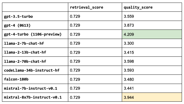

Sanity check: the retrieval scores are all the same because the LLM we choose doesn’t impact that part of our application.

Some of our LLMs have much larger context lengths, ex. gpt-4 is 8,192 tokens and gpt-3.5-turbo-16k is 16,384. We could increase the number of chunks that we use for these since we saw that increasing num_chunks continued to improve the retrieval and quality scores. However, we will keep this value fixed for now since the performance started to taper off anyway and so we can compare these performances under the exact same configurations.

1LLM = "mistralai/Mixtral-8x7B-Instruct-v0.1"

LinkLLM Cost analysis

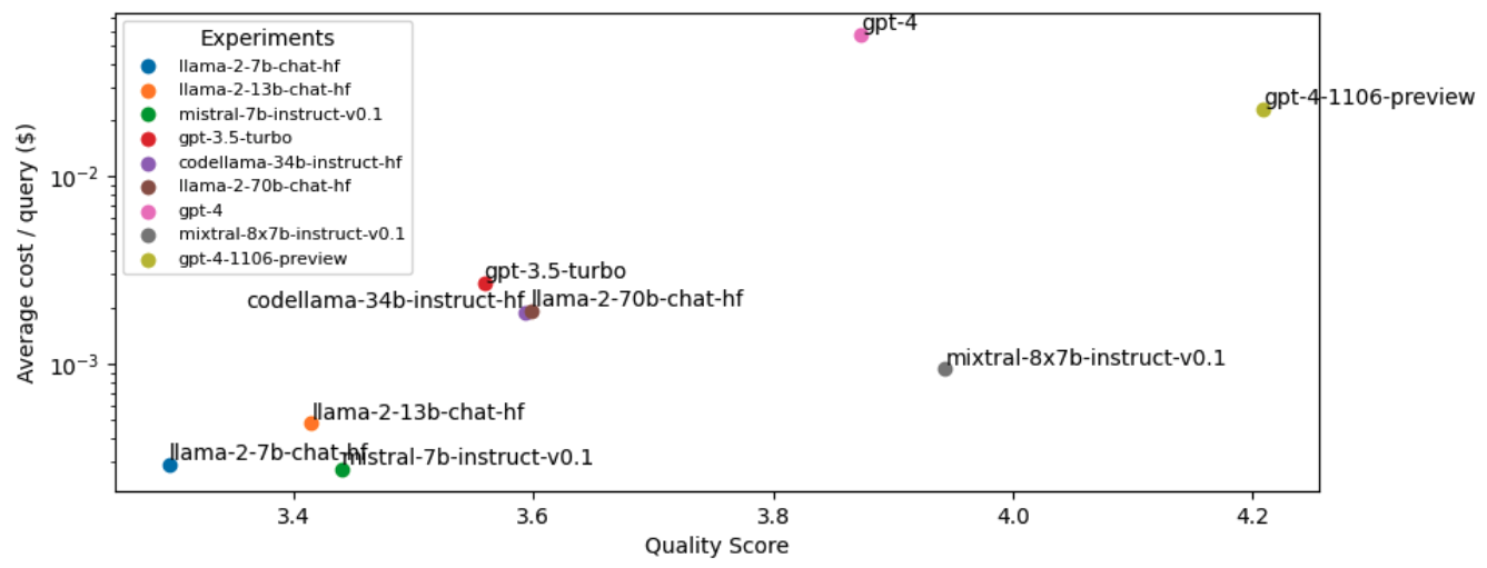
Besides just performance, we also want to evaluate the cost of our configurations (especially given the high price points of larger LLMs). We’re going to break this down into prompt and sampled pricing. The prompt size is the number of characters in our system, assistant and user contents (which includes the retrieved contexts). And the sampled size is the number of characters the LLM generated in its response.

Note: Our Llama-2 models are priced at $1/M tokens with Anyscale Endpoints.

1# Pricing per 1M tokens
2# Pricing per 1M tokens
3PRICING = {
4    "gpt-3.5-turbo": {
5        "prompt": 1.5,
6        "sampled": 2
7    },
8    "gpt-4": {
9        "prompt": 30,
10        "sampled": 60
11    },
12    "gpt-4-1106-preview": {
13        "prompt": 10,
14        "sampled": 30
15    },
16    "llama-2-7b-chat-hf": {
17        "prompt": 0.15,
18        "sampled": 0.15
19    },
20    "llama-2-13b-chat-hf": {
21        "prompt": 0.25,
22        "sampled": 0.25
23    },
24    "llama-2-70b-chat-hf": {
25        "prompt": 1,
26        "sampled": 1
27    },
28    "codellama-34b-instruct-hf": {
29        "prompt": 1,
30        "sampled": 1
31    },
32    "mistral-7b-instruct-v0.1": {
33        "prompt": 0.15,
34        "sampled": 0.15
35    },
36    "mixtral-8x7b-instruct-v0.1": {
37         "prompt": 0.50,
38         "sampled": 0.50
39    }
40}
41for llm in llms:
42    cost_analysis(llm=llm)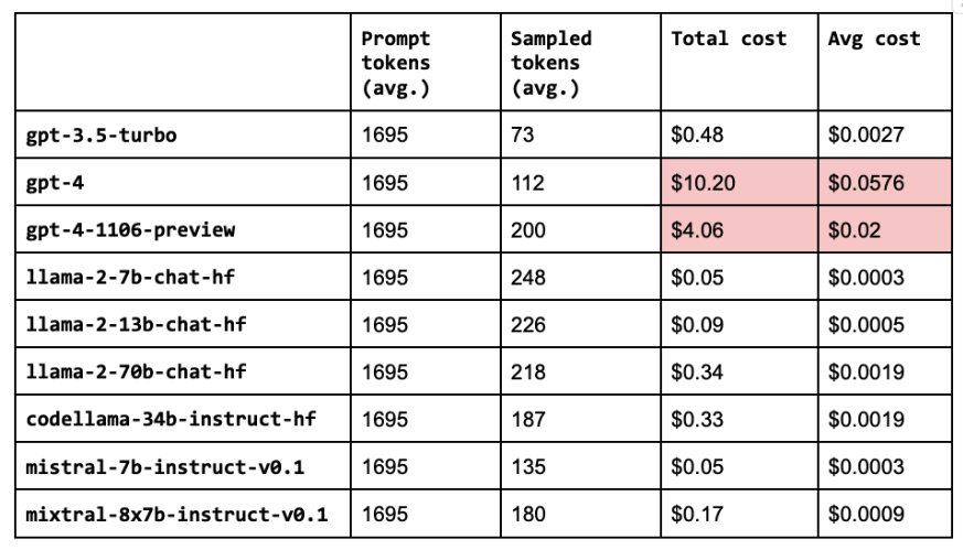

Link
Routing

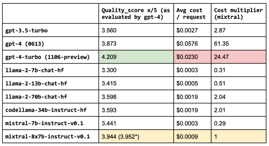
It seems that the most performant LLM, gpt-4, is also the most expensive one. While Llama-2-70b is very close in quality (without any fine-tuning yet) but about 47X more cost-effective than gpt-4 and 1.75X than gpt-3.5-turbo.

Note: In part 2 of this series, we’ll fine-tune our embedding models and OSS LLMs to make them even more performant.

However, we want to be able to serve the most performant and cost-effective solution. We can close this gap in performance between open source and proprietary models by routing queries to the right LLM according to the complexity or topic of the query. For example, in our application, open source models perform really well on simple queries where the answer can be easily inferred from the retrieved context. However, the OSS models fall short for queries that involve reasoning, numbers or code examples. To identify the appropriate LLM to use, we can train a classifier that takes the query and routes it to the best LLM.

Question for gpt-4:
{'question': 'if I am inside of a anyscale cluster how do I get my cluster-env-build-id', 'target': 0}
Question for Llama-2-70b:
{'question': 'what is num_samples in tune?', 'target': 1}

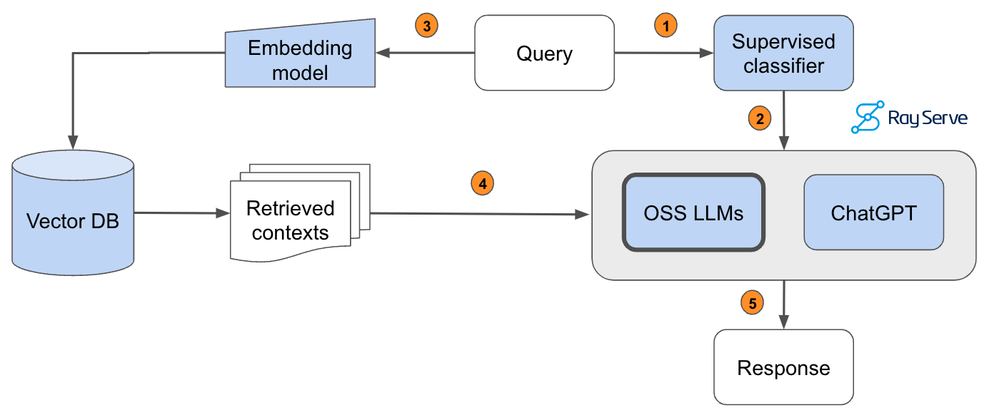
1. Pass the query to a supervised classifier that will determine which LLM is appropriate to answer it.

2. The predicted LLM receives the query.

3. Pass the query to our embedding model to semantically represent it.

4. Pass the retrieved context to the predicted LLM.

5. Generate the response.

In order to implement this, we hand-annotated a dataset of 1.8k queries according to which model (gpt-4 (label=0) or Llama-2-70b (label=1)) would be appropriate -- by default we route to Llama-2-70b and only if the query needs more advanced capabilities do we send the query to gpt-4. We then evaluate the performance of the model on a test dataset that has been scored with an evaluator.

1# Train classifier
2vectorizer = CountVectorizer()
3classifier = LogisticRegression(multi_class="multinomial", solver="lbfgs")
4router = Pipeline([("vectorizer", vectorizer), ("classifier", classifier)])
5router.fit(texts, labels)
6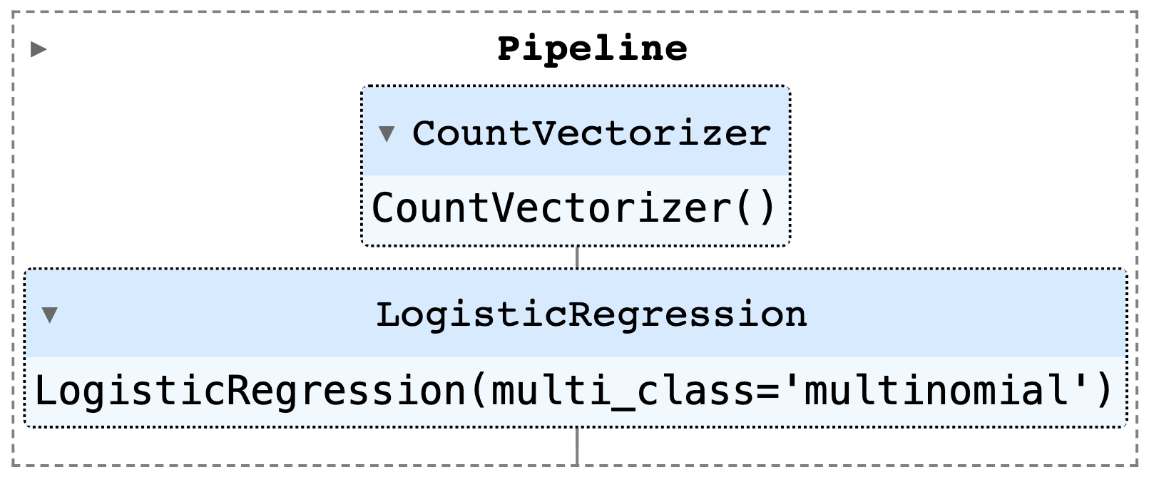

{
"precision": 0.917778649921507,
"recall": 0.9285714285714286,
"f1": 0.9215235703917096,
"num_samples": 574.0
}

# total samples 574
# samples for OSS models: 546 (95.1%)
Avg. score for samples predicted for Llama-2-70b: 3.8653846153846154
Avg. score for samples predicted for gpt-4: 3.625

Note: For our dataset, a small logistic regression model is good enough to perform the routing. But if your use case is more complex, consider training a more complex model, like a BERT-based classifier to perform the classification. These models are still small enough that wouldn’t introduce too much latency. Be sure to check out this guide if you want to learn how to train and deploy supervised deep learning models.

LinkServing

Now we're ready to start serving our Ray Assistant using our best configuration. We're going to use Ray Serve with FastAPI to develop and scale our service. First, we'll define some data structures like Query and Answer to represent the inputs and outputs to our service. We will also define a small function to load our index (assumes that the respective SQL dump file already exists). Finally, we can define our QueryAgent and use it to serve POST requests with the query. And we can serve our agent at any deployment scale we wish using the @serve.deployment decorator where we can specify the number of replicas, compute resources, etc.

1# Initialize application
2app = FastAPI()
3
4@serve.deployment(route_prefix="/", num_replicas=1, ray_actor_options={"num_cpus": 6, "num_gpus": 1})
5@serve.ingress(app)
6class RayAssistantDeployment:
7    def __init__(self, chunk_size, chunk_overlap, num_chunks, 
8                 embedding_model_name, embedding_dim,
9                 use_lexical_search, lexical_search_k, 
10                 use_reranking, rerank_threshold, rerank_k,
11                 llm, sql_dump_fp=None):
12
13        # Set up
14        chunks = build_or_load_index(
15            embedding_model_name=embedding_model_name, 
16            embedding_dim=embedding_dim, 
17            chunk_size=chunk_size, 
18            chunk_overlap=chunk_overlap,
19            sql_dump_fp=sql_dump_fp,
20        )
21
22        # Lexical index
23        lexical_index = None
24        self.lexical_search_k = lexical_search_k
25        if use_lexical_search:
26            texts = [re.sub(r"[^a-zA-Z0-9]", " ", chunk[1]).lower().split() for chunk in chunks]
27            lexical_index = BM25Okapi(texts)
28
29        # Reranker
30        reranker = None
31        self.rerank_threshold = rerank_threshold
32        self.rerank_k = rerank_k
33        if use_reranking:
34            reranker_fp = Path(EFS_DIR, "reranker.pkl")
35            with open(reranker_fp, "rb") as file:
36                reranker = pickle.load(file)
37
38        # Query agent
39        self.num_chunks = num_chunks
40        system_content = "Answer the query using the context provided. Be succinct. " \
41            "Contexts are organized in a list of dictionaries [{'text': <context>}, {'text': <context>}, ...]. " \
42            "Feel free to ignore any contexts in the list that don't seem relevant to the query. "
43        self.oss_agent = QueryAgent(
44            embedding_model_name=embedding_model_name,
45            chunks=chunks,
46            lexical_index=lexical_index,
47            reranker=reranker,
48            llm=llm,
49            max_context_length=MAX_CONTEXT_LENGTHS[llm],
50            system_content=system_content)
51        self.gpt_agent = QueryAgent(
52            embedding_model_name=embedding_model_name,
53            chunks=chunks,
54            lexical_index=lexical_index,
55            reranker=reranker,
56            llm="gpt-4",
57            max_context_length=MAX_CONTEXT_LENGTHS["gpt-4"],
58            system_content=system_content)
59
60        # Router
61        router_fp = Path(EFS_DIR, "router.pkl")
62        with open(router_fp, "rb") as file:
63            self.router = pickle.load(file)
64
65    @app.post("/query")
66    def query(self, query: Query) -> Answer:
67        use_oss_agent = self.router.predict([query.query])[0]
68        agent = self.oss_agent if use_oss_agent else self.gpt_agent
69        result = agent(
70            query=query.query, num_chunks=self.num_chunks, 
71            lexical_search_k=self.lexical_search_k, 
72            rerank_threshold=self.rerank_threshold, 
73            rerank_k=self.rerank_k, 
74            stream=False)
75        return Answer.parse_obj(result)

1# Deploy the Ray Serve application.
2deployment = RayAssistantDeployment.bind(
3    chunk_size=700,
4    chunk_overlap=50,
5    num_chunks=9,
6    embedding_model_name=os.environ["RAY_ASSISTANT_EMBEDDING_MODEL"],
7    embedding_dim=EMBEDDING_DIMENSIONS["thenlper/gte-large"],
8    use_lexical_search=False,
9    lexical_search_k=0,
10    use_reranking=True,
11    rerank_threshold=0.9,
12    rerank_k=9,
13    llm="mistralai/Mixtral-8x7B-Instruct-v0.1",
14    sql_dump_fp=Path(os.environ["RAY_ASSISTANT_INDEX"]))
15serve.run(deployment)

And with our application served, we’re ready to query it!

1# Inference
2data = {"query": "What is the default batch size for map_batches?"}
3response = requests.post("http://127.0.0.1:8000/query", json=data)
4print(response.text)
5

{
'question': 'What is the default batch size for map_batches?',  
'sources': ['https://docs.ray.io/en/master/data/api/doc/ray.data.Dataset.map_batches.html#ray-data-dataset-map-batches', 'https://docs.ray.io/en/master/data/transforming-data.html#configuring-batch-size', 'https://docs.ray.io/en/master/data/data-internals.html#execution-memory', 'https://docs.ray.io/en/master/serve/advanced-guides/dyn-req-batch.html#tips-for-fine-tuning-batching-parameters', 'https://docs.ray.io/en/master/data/examples/pytorch_resnet_batch_prediction.html#model-inference', 'https://docs.ray.io/en/master/data/batch_inference.html#configuring-batch-size', 'https://docs.ray.io/en/master/data/examples/huggingface_vit_batch_prediction.html#step-3-scaling-up-to-the-full-dataset-with-ray-data'], 
'answer': 'The default batch size for map_batches is 4096.', 
'llm': 'meta-llama/Llama-2-70b-chat-hf'
}

Note: As we can see, Ray Serve makes model composition extremely easy and we could continue to make this even more fine-grained. For example, we can train a classifier to discern between queries for Llama-2-70b, CodeLlama-34b-Instruct-hf (for code generation) and gpt-4 (for highly complex queries).

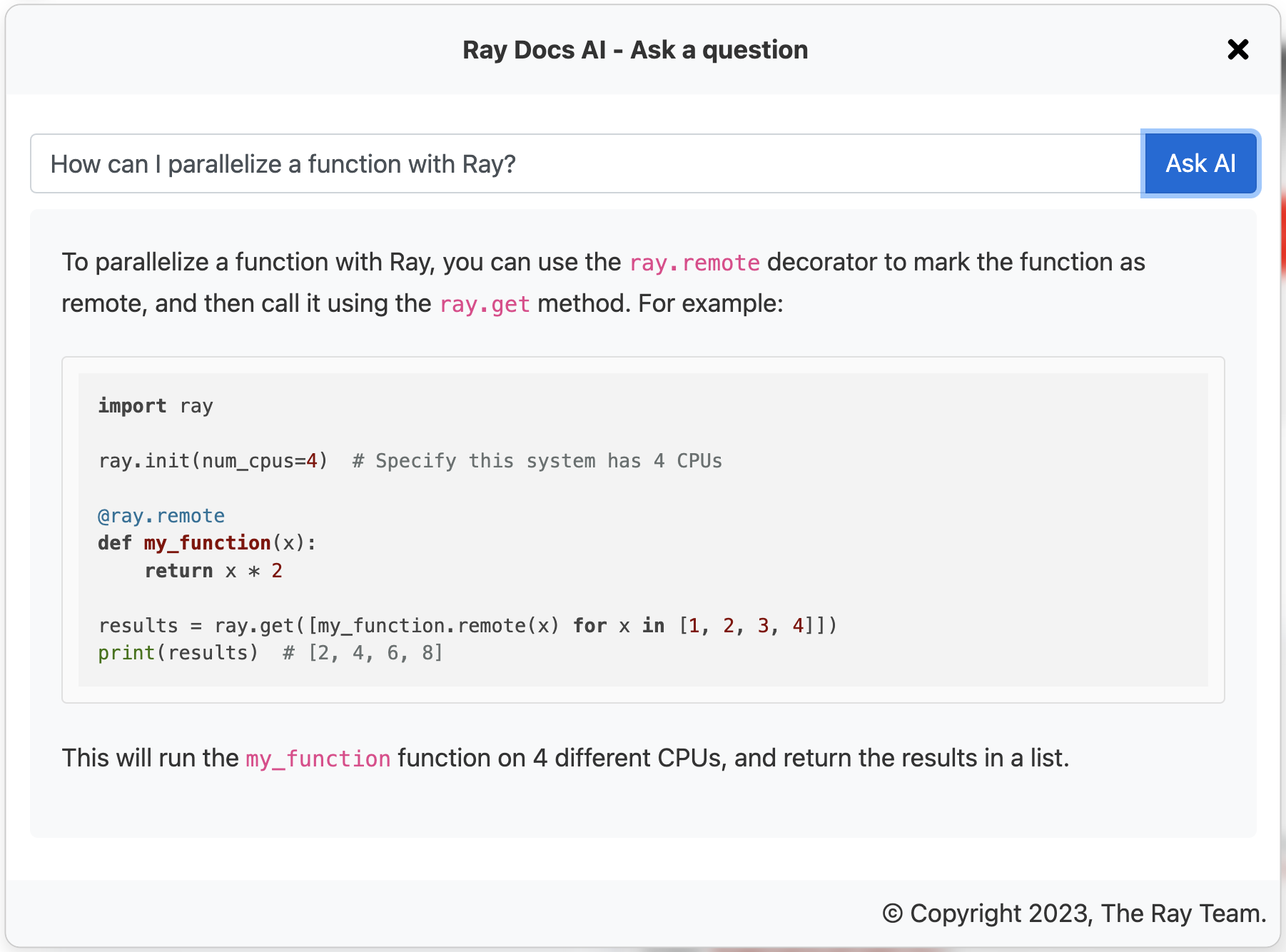
Once our application is served, we’re free to use it anywhere we want. For example, we use it as a bot on our Slack channels and as a widget on our docs page (public release coming soon). We can use this to collect feedback from our users to continually improve the application (fine-tuning, UI/UX, etc.).

LinkImpact

Link1st order

Building an LLM application like this has had a tremendous impact on our products and company. There were expected 1st order impacts in overall developer and user adoption for our products. The capability to interact and solve problems that our users experience in a self-serve and immediate manner is the type of feature that would improve the experience of any product. It makes it significantly easier for people to succeed and it elevated the perception around LLM applications from a nice-to-have to a must-have. 

Link2nd order

However, there were also some 2nd order impacts that we didn’t immediately realize. For example, when we further inspected user queries that yielded poor scores, often the issue existed because of a gap in our documentation. When we made the fix (ex. added the appropriate section to our docs), this improved our product and the LLM application itself — creating a very valuable feedback flywheel. Furthermore, when internal teams learned of the capabilities of our LLM application, this generated the development of highly valuable LLM applications that depend on this Ray docs LLM application as one of its foundational agents that it uses to perform its tasks. 

For example, we’ve internally developed a feature called Anyscale Doctor that helps developers diagnose and debug issues during development. Issues in code can be caused by a variety of reasons but when the issue is Ray related, the LLM application we built here is called to aid in resolving the particular issue.

LinkNext steps

In the next guide, we’ll discuss how we continuously keep our RAG application up to date as our data sources grow and how to leverage the feedback from production to fine-tune our embedding models and LLMs.

• add additional context with retrieved chunks

• keyword search with semantic (embedding) search

• reranking with LLM on retrieved chunks (from embeddings)

• fine-tune embedding model

• fine-tune base LLM (OSS) with Anyscale Endpoints

• longer context lengths (RoPE)

• structuring and updating the index in the vector DB

• offline/online indexing of new data

LinkLearn more

• If your team is investing heavily in developing LLM applications, reach out to us to learn more about how Ray and Anyscale can help you scale and productionize everything.

• Starting serving (+fine-tuning) OSS LLMs with Anyscale Endpoints ($1/M tokens for Llama-2-70b) and private endpoints available upon request (1M free tokens trial).

• Learn more about how companies like OpenAI, Netflix, Pinterest, Verizon, Instacart and others leverage Ray and Anyscale for their AI workloads at the Ray Summit 2023 this Sept 18-20 in San Francisco